Recurrent Neural Networks (RNNs) and LSTMs for Time Series Forecasting

In our last article we reviewed time series forecasting with TensorFlow using a simple deep neural network. In this article, we'll expand on this by using sequence models such as recurrent neural networks (RNNs) and LSTMs for time series forecasting.

RNNs and LSTMs are useful for time series forecasting since the state vector and the cell state allow you to maintain context across a series. In other words, they allow you to carry information across a larger time window than simple neural networks.

RNNs and LSTMs can also apply different weights to sequences of data, meaning they are often better at weighting the importance of recent data more heavily than data further in the past.

We'll also look at how we can use Lambda layers in our neural networks, which allow us to add arbitrary operations to our models to expand the functionality of TensorFlow and Keras.

This article is based on notes from this course on Sequences, Time Series and Prediction and is organized as follows:

• Review of Recurrent Neural Networks (RNNs)
• Shape of Inputs to an RNN
• Outputting a Sequence
• Lambda Layers
• Adjusting the Learning Rate Dynamically
• LSTMs for Time Series Forecasting
• Convolutional Layers for Time Series Forecasting

This post may contain affiliate links. See our policy page for more information.

Review of Recurrent Neural Networks (RNNs) & LSTMS

We won't cover RNNs and LSTMs in detail in this article, although here is a brief review from our Introduction to Recurrent Neural Networks & LSTMs:

A recurrent neural network (RNN) attempts to model time-based or sequence-based data. An LSTM network is a type of RNN that uses special units as well as standard units.

RNNs contain recurrent layers that are designed to process sequences of inputs. You can feed in batches of sequences into RNNs and it will output a batch of forecasts after going through a dense layer.

One difference from our simple DNNs in the previous article is that the full input shape when using RNNs is three dimensional. The first dimension will be the batch size, the second will be the number of time steps, and the third is the dimensionality of the inputs at each time step.

The recurrent layers uses a memory cell at each time step, which takes the input value $X_0$ and calculates the output for that step $\hat{Y_0}$ and a state vector $H_0$ thats fed into the next step.

This process repeats to produce $X_1$, $\hat{Y_1}$, $H_1$, and so on, until we reach the end of our input dimension. This is what gives this architecture the name recurrent neural network because the values recur due to the output of the cell being fed back into the next cell.

Shape of Inputs to an RNN

As mentioned, the shape of an RNNs inputs are three dimensional. If we have a window size of 30 time steps and we batch them in sizes of four, the shape will be 4 x 30 x 1 = 120.

At each time step the memory cell input will be a four by one matrix. The cell will also take the input of the state matrix from the previous step. In addition to the state vector, the cell will output a $Y$ value.

If the memory cell has three neurons, the output matrix will be 4 by 3 since the batch size coming in was four and the number of neurons is three. In this case, the output of the layer would be 4 by 30 by 3, where 4 is the batch size, 30 is the number of time steps, and 3 being the number of units.

In a simple RNN, $H_0$ is a copy of the output matrix $Y$, which means that $H_0$ is a copy of $\hat{Y_0}$, $H_1$  is a copy of $\hat{Y_1}$, and so on. This means that at each time step the memory cell gets both the current input and the previous output.

In some cases we may want a single vector for each instance in the batch, which is referred to as a Sequence-to-Vector RNN. These ignore all of the outputs except for the last one. This is the default when using Keras and TensorFlow, so if we want a recurrent layer to output a sequence we need to specify return_sequences=True when creating the layer.

Outputting a Sequence

Below is an example of an RNN with two recurrent layers:

• The first layer has return_sequences=True which is fed into the next layer
• Notice that the input_shape=[None, 1]—TensorFlow assumes the first dimension is the batch_size which can have any size so you don't need to define it. The next dimension is the number of time steps, which we can set to None meaning that the RNN can handle any length of sequence. The final dimension is 1 because we have a univariate time series.
• The next layer also return_sequences set to True, so it will output a sequence to the denser layer.
• This is referred to as a sequence-to-sequence RNN, which is fed a batch of sequences and returns a batch of sequences of the same length
• If we remove the return_sequences=True from the second layer this would output to a single dense layer

model = keras.models.Sequential([
                                 keras.layers.SimpleRNN(20, return_sequences=True,
                                                        input_shape=[None, 1]),
                                 keras.layers.SimpleRNN(20, return_sequences=True),
                                 keras.layers.Dense(1)
])

Lambda Layers

Next, we'll add several lambda layers to the RNN, which allow us to add arbitrary operations to expand the functionality of Keras:

• The first lambda layer helps expands our dimensionality—here we are expanding the array by 1 dimension and by setting input_shape=[None], which means the model can take sequences of any length
• The final lambda layer is scaling the outputs by 100, which can help training. The default layer in the RNN is tanh, which outputs values between -1 and 1. By scaling the outputs we can make these values closer to our time series, which are usually values in the 40s, 50s, 60s, and so on.

model = keras.models.Sequential([
                                 keras.layers.Lambda(lambda x: tf.expand_dims(x, axis=-1),
                                                     input_shape=[None]),
                                 keras.layers.SimpleRNN(20, return_sequences=True,
                                                        input_shape=[None, 1]),
                                 keras.layers.SimpleRNN(20, return_sequences=True),
                                 keras.layers.Dense(1),
                                 keras.layers.Lambda(lambda x: x * 100.0)
])

Adjusting the Learning Rate Dynamically

Now that we've looked at sequence-to-vector and sequence-to-sequence RNNs, let's see how useful they are for time series forecasting.

We're first going to optimize the neural network's learning rate of the optimizer dynamically, which can save a lot of time in hyperparameter tuning.

Below is the code to train a simple RNN with two layers, each with 40 cells:

• To dynamically tune the learning rate we set up a callback using the LearningRateScheduler
• It uses a new loss function called Huber, which is less sensitive to outliers

train_set = windowed_dataset(x_train, window_size, batch_size=128, shuffle_buffer=shuffle_buffer_size)

model = tf.keras.models.Sequential([
  tf.keras.layers.Lambda(lambda x: tf.expand_dims(x, axis=-1),
                      input_shape=[None]),
  tf.keras.layers.SimpleRNN(40, return_sequences=True),
  tf.keras.layers.SimpleRNN(40),
  tf.keras.layers.Dense(1),
  tf.keras.layers.Lambda(lambda x: x * 100.0)
])

lr_schedule = tf.keras.callbacks.LearningRateScheduler(
    lambda epoch: 1e-8 * 10**(epoch / 20))
optimizer = tf.keras.optimizers.SGD(lr=1e-8, momentum=0.9)
model.compile(loss=tf.keras.losses.Huber(),
              optimizer=optimizer,
              metrics=["mae"])
history = model.fit(train_set, epochs=100, callbacks=[lr_schedule])

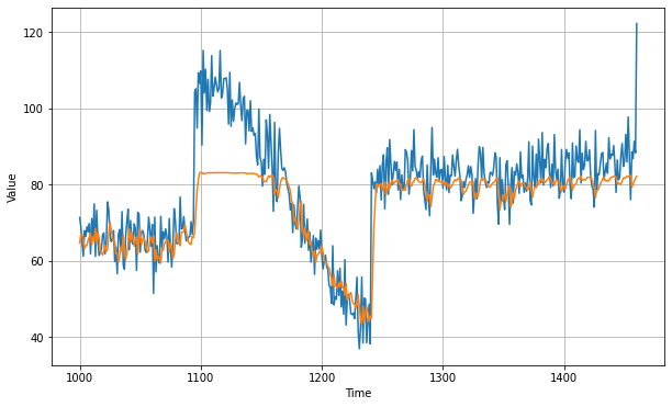
After training for 400 epochs we get an MAE of roughly 6.82:

You can find the code for this RNN on Laurence Moroney's Github here. This was just a simple RNN, let's now look at how we can improve this with an LSTM.

LSTMs for Time Series Forecasting

Recall that RNNs have cells that take batches of inputs, or $X$, and calculated a $Y$ output and a state vector. The state vector and the next $X$ are then fed into the next cell, which result in the next $Y$, and so on.

While the state is a factor in subsequent calculations, its impact can diminish significantly over time. To solve this, LSTMs add a memory cell state which keeps a state from time step to step throughout throughout the training cycle.

This memory cell means that data from earlier in the time series can have a greater impact than RNNs on the overall prediction. This cell can also be bidirectional so the state moves forward and backward.

You can learn more about LSTMs from Andrew Ng's course on Sequence Models here.

Below is an update to our previous RNN. After the first Lambda layer that expands the dimensions, there are two bidirectional LSTM layer with 32 cells:

tf.keras.backend.clear_session()
dataset = windowed_dataset(x_train, window_size, batch_size, shuffle_buffer_size)

model = tf.keras.models.Sequential([
  tf.keras.layers.Lambda(lambda x: tf.expand_dims(x, axis=-1),
                      input_shape=[None]),
   tf.keras.layers.Bidirectional(tf.keras.layers.LSTM(32, return_sequences=True)),
  tf.keras.layers.Bidirectional(tf.keras.layers.LSTM(32)),
  tf.keras.layers.Dense(1),
  tf.keras.layers.Lambda(lambda x: x * 100.0)
])


model.compile(loss="mse", optimizer=tf.keras.optimizers.SGD(lr=1e-5, momentum=0.9),metrics=["mae"])
history = model.fit(dataset,epochs=500,verbose=0)

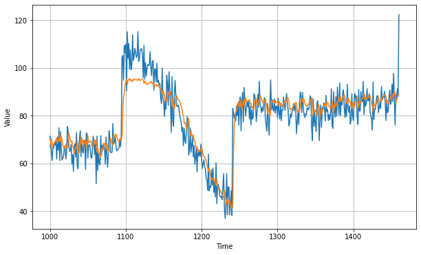
With this LSTM model we get an improved MAE of roughly 5.45:

You can find the code for this LSTM on Laurence Moreney's Github here. Next, we'll look at how adding a convolutional layer impacts the results of the time series prediction.

Convolutional Layers for Time Series

As discussed, RNNs and LSTMs are useful for learning sequences of data. Let's now look at how we can improve this further by adding a convolutional layer.

Below is the model we've been working with, although with a one dimensional convolutional layer before the LSTM layers:

• We use a Conv1D that tries to learn 32 filters
• It is 1 dimensional so we use a 3 numbered window and multiply the values in the window by the filter values, which is similar to how image convolutions are calculated
• The Lambda layer that reshaped the input layer has been removed, and instead we specify an input_shape=[None, 1] on the Conv1D. This means that we still need to update the windowed_dataset helper function with tf.expand_dims

model = tf.keras.models.Sequential([
  tf.keras.layers.Conv1D(filters=32, kernel_size=3,
                      strides=1, padding="causal",
                      activation="relu",
                      input_shape=[None, 1]),
  tf.keras.layers.LSTM(32, return_sequences=True),
  tf.keras.layers.LSTM(32, return_sequences=True),
  tf.keras.layers.Dense(1),
  tf.keras.layers.Lambda(lambda x: x * 200)
])

optimizer = tf.keras.optimizers.SGD(lr=1e-5, momentum=0.9)
model.compile(loss=tf.keras.losses.Huber(),
              optimizer=optimizer,
              metrics=["mae"])
history = model.fit(dataset,epochs=500)

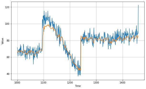
As you can see below, by stacking the CNN with an LSTM, after 500 epochs we were able to create the best forecast yet with an MAE of roughly 5:

You can find the code for this notebook on Laurence Moroney's Github here.

Summary: RNNs and LSTMs for Time Series Forecasting

As discussed, RNNs and LSTMs are highly useful for time series forecasting as the state vector and cell state allow the model to maintain context across a series. In particular, these features of sequence models allow you to carry information across a larger time window than simple deep neural networks.

We also reviewed how we can use Lambda layers to add arbitrary operations to our TensorFlow and Keras models. Finally, we looked at how we can stack a convolutional layer before an LSTM layer to improve model performance.

Resources

• Sequences, Time Series and Prediction