Time Series with TensorFlow: Downloading & Formatting Historical Bitcoin Data

In this series of articles, we're going to discuss how to use TensorFlow for time series data.

Time series data refers to any data that has a time component, examples of which include:

• Forecasting stock prices
• Predicting energy consumption levels
• Analyzing ECG data to detect heartbeat irregularities, and so on

For this series, we'll work with historical Bitcoin price data and build several models with TensorFlow to predict future prices.

Of course, the goal of this project is not to build the ultimate AI-based trading algorithm, instead, it's to understand the process of working through time-series data problems with TensorFlow.

As always, this is not financial advice, past performance is not indicative of future results, and you should not use these models in the real world. See our full Terms of Service for more information.

This series of articles is based on notes from this TensorFlow Developer Certificate course and is organized as follows:

• Time series inputs and outputs
• Importing time series data with Python's CSV module
• Importing time series data with Pandas
• Visualizing historical Bitcoin data with Pandas
• Creating train and test sets for time series data

Time series inputs and outputs

For this project, the question we'll be trying to answer is "what will the price of Bitcoin be tomorrow?".

This means that the output of our model will be a price forecast, in other words, the output of our model will be continuous.

If we were trying to model whether the price would go up or down, this would be a classification problem and the output would be discrete.

In order to produce this output, we the first step is to numerically encode our input data. The good thing about time series data, however, is that it's often already numerical.

For this project, we want our input to be a previous period of price data, let's say the previous week of price data, and the output will be the next's days price prediction.

More specifically, we'll pass our model a window of one week of Bitcoin price data in order to predict the next day's price. For time series data, the predicted time period is often referred to as the horizon.

We'll discuss this more later, but here are the specific inputs and output shapes we'll be working with:

• Input: [batch_size, window_size] shape is is [None, 7] or [32, 7]
• Output: [horizon] shape is [1]

Given this, we can frame this as a sequence (seq2seq) problem, or a many-to-one problem as Andrej Karpathy highlights:

Importing time series data with Python's CSV module

Let's now create a new Colab notebook for the project. After that, the first step will be the import the data we'll be working with.

There are a number of places to get Bitcoin price data, although for this project we'll use the daily price data from Yahoo Finance. Note this data only goes back to September 14, 2014, although that will work for demonstration purposes.

To import our data with Python's CSV module, we'll create an empty list called timesteps that will store our dates and btc_price that will store the price of Bitcoin.

We'll then upload our CSV file into Colab and import it as follows:

# Import and format historical Bitcoin data with Python
import csv
from datetime import datetime

timesteps = []
btc_price = []
with open("/content/BTC-USD.csv", "r") as f:
  csv_reader = csv.reader(f, delimiter=",")
  next(csv_reader) # skipe the column titles line
  for line in csv_reader:
    timesteps.append(datetime.strptime(line[0], "%Y-%m-%d")) # get the dates as dates, not strings
    btc_price.append(float(line[4])) # get the closing price as a float

# View first 10 of each
timesteps[:10], btc_price[:10]

Importing time series data with Pandas

Another way we can import our data is with Pandas, we just need to parse the dates, and set the index_col to Date since we're working with time series data:

# import with pandas
import pandas as pd
# Read in Bitcoin data and parse the dates
df = pd.read_csv("/content/BTC-USD.csv",
                 parse_dates=["Date"],
                 index_col=["Date"])
df.head()

Let's now familiarize ourselves with the data with df.info() and check how many samples we have with len(df). We can see there are 2945 samples in this dataset.

As you may know, deep learning models work best when there a lot of samples train on, typically this is tens of thousands, millions, or tens of millions depending on the size of the project.

With time series data, however, we'll often run into a smaller number of samples to work with.

In this case, we're just working with daily data, although if we wanted to increase the number of samples we could simply change the time frame to hourly, minute, or even second-level tick data.

Visualizing historical Bitcoin data with Pandas

The next step in any machine learning project is to visualize the data.

To start, let's reduce the dataframe to just the daily closing price and rename the column to Price:

bitcoin_prices = pd.DataFrame(df["Close"]).rename(colums={"Close": "Price"})

Next, we'll import matplotlib and visualize the daily prices:

import matplotlib.pyplot as plt
bitcoin_prices.plot(figsize=(10, 7))
plt.ylabel("BTC Price")
plt.title("Bitcoin Price from Sept 14, 2014 to Oct 09, 2022", fontsize=16)
plt.legend(fontsize=14)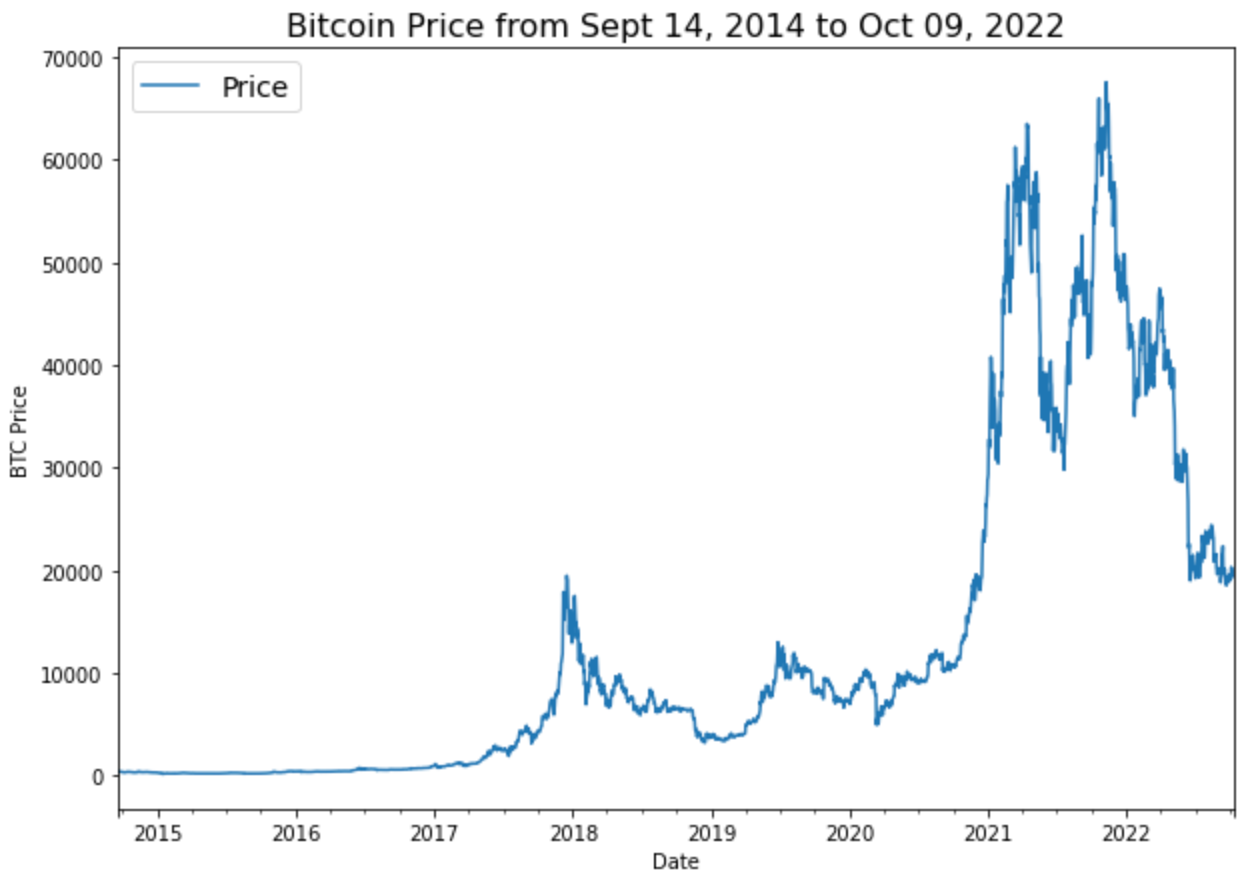

Creating train and test sets for time series data

Next, let's create train and test datasets for our models.

Unlike other machine learning problems, with time series data we can't randomly split the data and instead need to choose a specific cutoff date for the training and test sets.

Before we split the data, let's first turn the timesteps and Price into an array:

# Get bitcoin date array
timesteps = bitcoin_prices.index.to_numpy()
prices = bitcoin_prices["Price"].to_numpy()

Next, let's split the data into 80% for training and 20% for testing:

# Create train and test sets
split_size = int(0.8 * len(prices)) # 80% train, 20% test

# Create train data splits
X_train, y_train = timesteps[:split_size], prices[:split_size]

# Create test data splits
X_test, y_test = timesteps[split_size:], prices[split_size:]

Next, we'll visualize our training and test data:

# Plot train and test split
plt.figure(figsize=(10,7))
plt.scatter(X_train, y_train, s=5, label="Train data")
plt.scatter(X_test, y_test, s=5, label="Test data")
plt.xlabel("Date")
plt.ylabel("BTC Price")
plt.legend(fontsize=14)
plt.show;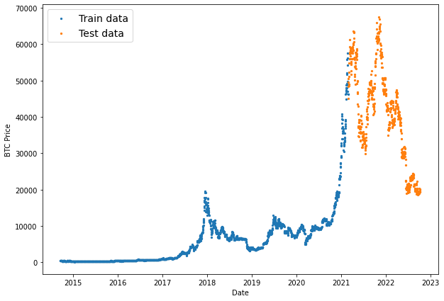

Create a plotting function to visualize our data

Before we start creating forecasting models, let's create a plotting function to make visualizing our time series data less tedious:

# Create a function to plot time series data
def plot_time_series(timesteps, values, format=".", start=0, end=None, label=None):
  # plot the series
  plt.plot(timesteps[start:end], values[start:end], format, label=label)
  plt.xlabel("Time")
  plt.ylabel("BTC Price")
  if label:
    plt.legend(fontsize=14)
  plt.grid(True)

# test our plotting function
plt.figure(figsize=(10,7))
plot_time_series(timesteps=X_train, values=y_train, label="Train Data")
plot_time_series(timesteps=X_test, values=y_test, label="Test Data")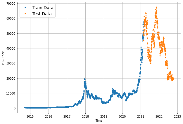

Summary: Time Series with TensorFlow

In this article, we started a new Time Series with TensorFlow project by importing our data into Colab with both Python's CSV module and Pandas.

We then visualized the data, formatted it into train and test sets, and finally created a plotting function to make visualizing the data less tedious in the future.

In the next article, we'll discuss the various modeling experiments that we'll be running and start creating a naive forecasting model.

Resources

• TensorFlow Developer Certificate course