Machine Learning

Time Series with TensorFlow: Building an LSTM (RNN) for Forecasting

In this Time Series with TensorFlow article, we build a recurrent neural network (LSTM) model for forecasting Bitcoin price data.

2 years ago • 5 min read

By Peter Foy

In our previous Time Series with TensorFlow article, we built a 1-dimensional convolutional neural network (Conv1D) and compared it to the performance of our previous dense and naive models.

In this article, we'll continue testing new models for the task of Bitcoin price forecasting and an LSTM recurrent neural network (RNN). In our previous guide Introduction to Recurrent Neural Networks & LSTMs, we highlighted that:

A recurrent neural network attempts to model time-based or sequence-based data.An LSTM network is a type of RNN that uses special units as well as standard units.

This article is based on notes from this TensorFlow Developer Certificate course and is organized as follows:

Model 5: LSTM (RNN)
Evaluating model 5

Previous articles in this series can be found below:

Stay up to date with AI

Model 5: LSTM (RNN)

Instead of discussing the theory of LSTM and RNNs, we're just going to jump into model building.

Previously we've been using the Sequential API from TensorFlow which is useful for a sequential stack of layers. TensorFlow also has the Functional API, which allows a bit more flexibility with the models you're building so we'll use that for our LSTM.

Here are the docs for a TensorFlow LSTM layer, which we can see takes as input a 3D tesnor with shape [batch, timesteps, feature]. This means we don't need to recreate our data from our previous CNN model since it has the same input shape.

Also, to keep in line with the theme of creating the simplest possible models and then adding complexity as needed, we're going to just create a 1 layer LSTM.

tf.random.set_seed(42)

# Build an LSTM with the Functional API
inputs = layers.Input(shape=WINDOW_SIZE)
x = layers.Lambda(lambda x: tf.expand_dims(x, axis=1))(inputs)
x = layers.LSTM(128)(x)
output = layers.Dense(HORIZON)(x)
model_5 = tf.keras.Model(inputs=inputs, outputs=output, name="model_5_LSTM")

# Compile model
model_5.compile(loss="mae", optimizer=tf.keras.optimizers.Adam())

# Fit model
model_5.fit(train_windows,
            train_labels,
            epochs=100,
            verbose=1,
            batch_size=128,
            validation_data=(test_windows, test_labels),
            callbacks=[create_model_checkpoint(model_name=model_5.name)])

Immediately we can see the loss is significantly worse than previous models and not getting better as it's training, so let's pause this and add two more layers to our model - another LSTM layer and a dense layer:

tf.random.set_seed(42)

# Build an LSTM with the Functional API
inputs = layers.Input(shape=WINDOW_SIZE)
x = layers.Lambda(lambda x: tf.expand_dims(x, axis=1))(inputs)
x = layers.LSTM(128, return_sequences=True)(x)
x = layers.LSTM(128)(x)
x = layers.Dense(32, activation="relu")(x)
output = layers.Dense(HORIZON)(x)
model_5 = tf.keras.Model(inputs=inputs, outputs=output, name="model_5_LSTM")

# Compile model
model_5.compile(loss="mae", optimizer=tf.keras.optimizers.Adam())

# Fit model
model_5.fit(train_windows,
            train_labels,
            epochs=100,
            verbose=1,
            batch_size=128,
            validation_data=(test_windows, test_labels),
            callbacks=[create_model_checkpoint(model_name=model_5.name)])

Even with these new layers the loss is still very high...so what's going wrong?

In this case, the issue is that we're using the default LSTM layers that TensorFlow provides. Typically, these default layers work quite well, but let's try adjusting the activation function from the default tanh to relu.

We'll also remove the dense layer and just use LSTM layers for now:

tf.random.set_seed(42)

# Build an LSTM with the Functional API
inputs = layers.Input(shape=WINDOW_SIZE)
x = layers.Lambda(lambda x: tf.expand_dims(x, axis=1))(inputs)
x = layers.LSTM(128, return_sequences=True)(x)
x = layers.LSTM(128, activation="relu")(x)
output = layers.Dense(HORIZON)(x)
model_5 = tf.keras.Model(inputs=inputs, outputs=output, name="model_5_LSTM")

# Compile model
model_5.compile(loss="mae", optimizer=tf.keras.optimizers.Adam())

# Fit model
model_5.fit(train_windows,
            train_labels,
            epochs=100,
            verbose=1,
            batch_size=128,
            validation_data=(test_windows, test_labels),
            callbacks=[create_model_checkpoint(model_name=model_5.name)])

Evaluating model 5

Let's now load in the best performing model and evaluate it on our test data:

# Load in best performing model & evaluate on test data
model_5 = tf.keras.models.load_model("model_experiments/model_5_LSTM")
model_5.evaluate(test_windows, test_labels)

We can still this is still a much higher loss than our previous CNN model, but let's still make predictions with our LSTM model:

# Make predictions with LSTM model
model_5_preds = make_preds(model_5, test_windows)
model_5_preds[:5]

Let's evaluate model 5 predictions:

# Evaluate model 5 predictions
model_5_results = evaluate_preds(y_true=tf.squeeze(test_labels),
                                 y_pred=model_5_preds)
model_5_results

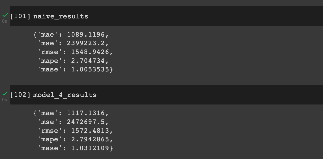
We see the LSTM in its current architecture is performing slightly worse than both the naive results and our previous CNN model and our first simple dense model.

Again, there's much more we could do with hyperparameter tuning to improve our LSTM, but this highlights another important point in machine learning, namely:

Neural networks are powerful algorithms that can be applied to almost any problem, although that doesn't always mean they'll achieve superior results to simpler statistical models.

Now that we've built several models with univariate input, meaning only price data as input, let's move on to building several models with multivariate data.

Summary: Building an LSTM for forecasting

In this article, we'll continue testing new models for the task of Bitcoin price forecasting and an LSTM recurrent neural network (RNN). An LSTM network is a type of recurrent neural network that uses special units as well as standard units.

As we saw, our model still hasn't been able to perform better than our simple dense models or our initial naive model.

In the next article, we'll begin to with multivariate data for the task of time series forecasting.