Introduction to Sequences and Time Series Forecasting with TensorFlow

In this article, we'll look at how to build time series forecasting models with TensorFlow, including best practices for preparing time series data.

These models can be used to predict a variety of time series metrics such as stock prices or forecasting the weather on a given day. We'll also look at how to create a synthetic sequence of data to understand the common attributes of time series data such as trends, seasonality, and noise.

This article is based on notes from course 4 of the TensorFlow Developer Certificate Program and is organized as follows:

• Review of Time Series Data
• Machine Learning for Time Series Data
• Common Patterns in Time Series Data
• Introduction to Time Series with Python
• Train, Validation, and Test Sets
• Metrics to Evaluate Performance
• Moving Average and Differencing
• Machine Learning Techniques for Time Series Forecasting
• Feeding a Windowed Dataset into a Neural Network
• Single Layer Neural Network for Forecasting
• Deep Neural Network for Forecasting

This post may contain affiliate links. See our policy page for more information.

Review of Time Series Data

A time series is defined as an ordered sequence of values that are typically evenly spaced over time. Time series data can be broken into the following categories:

• Univariate time series: There is a single value recorded sequentially over equal time increments.
• Multivariate time series: There are multiple values at each time step. These can be analyzed to understand relationships between multiple variables.

Machine Learning for Time Series Data

In the context of machine learning for time series, one application is prediction or forecasting based on past data.

In some cases, we can also project back into the past in order to better understand the current data. This process is called imputation, which is the process of replacing missing data with substituted values.

Another application of machine learning for time series data is anomaly detection, which is the identification of outliers or rare items that differ significantly from the majority of data.

Common Patterns in Time Series Data

There are a number of common patterns that frequently come up in time series data, these include:

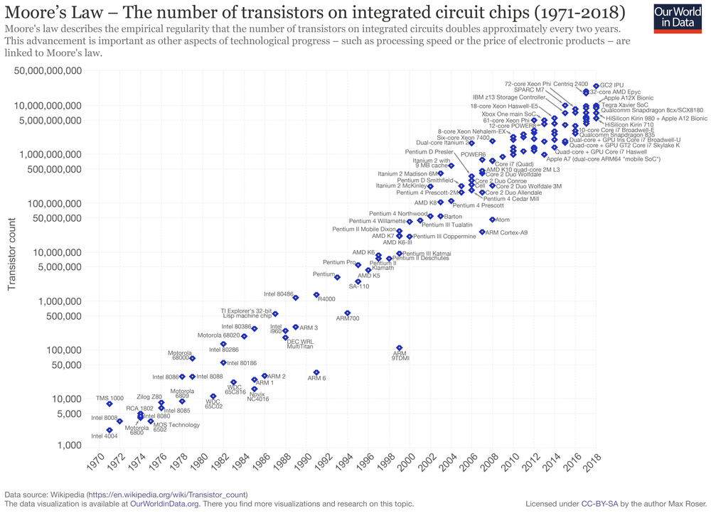
• Trends: This means the time series has a specific direction it's moving in. For example, Moore's law clearly has an upward trend in the number of transistors over time:

• Seasonality: This means that patterns repeat in predictable intervals. For example, active users of a website will often experience predictable dips on the weekends.
• White Noise: Time series data can also be completely random, which is referred to as noise. As MachineLearningMastery puts it:

A time series is white noise if the variables are independent and identically distributed with a mean of zero. This means that all variables have the same variance (sigma^2) and each value has a zero correlation with all other values in the series.

• Autocorrelated: This means the data correlates with a delayed copy of itself, which is often called a lag. As Investopedia puts it

Autocorrelation represents the degree of similarity between a given time series and a lagged version of itself over successive time intervals.

Time series data in real life will typically have have a combination of seasonality, trend, autocorrelation, and noise.

Introduction to Time Series with Python

Let's now review these common attributes of a time series with a synthetic example using Python. Here's how we can create a simple upward trend with Python, NumPy, and Matplotlib:

import numpy as np
import matplotlib.pyplot as plt
import tensorflow as tf
from tensorflow import keras

def plot_series(time, series, format="-", start=0, end=None, label=None):
    plt.plot(time[start:end], series[start:end], format, label=label)
    plt.xlabel("Time")
    plt.ylabel("Value")
    if label:
        plt.legend(fontsize=14)
    plt.grid(True)

def trend(time, slope=0):
    return slope * time

time = np.arange(4 * 365 + 1)
baseline = 10
series = trend(time, 0.1)

plt.figure(figsize=(10, 6))
plot_series(time, series)
plt.show()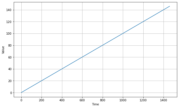

Next, we can generate seasonality with Python as follows:

def seasonal_pattern(season_time):
    return np.where(season_time < 0.4,
                    np.cos(season_time * 2 * np.pi),
                    1 / np.exp(3 * season_time))

def seasonality(time, period, amplitude=1, phase=0):
    season_time = ((time + phase) % period) / period
    return amplitude * seasonal_pattern(season_time)

baseline = 10
amplitude = 40
series = seasonality(time, period=365, amplitude=amplitude)

plt.figure(figsize=(10, 6))
plot_series(time, series)
plt.show()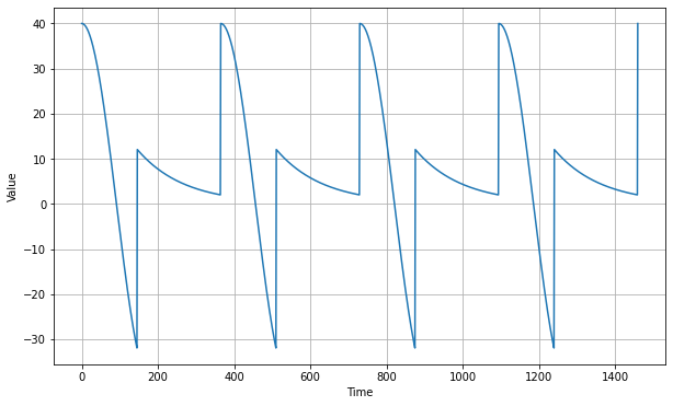

In order to add noise we can use the white_noise function below and plot it in our seasonal time series:

def white_noise(time, noise_level=1, seed=None):
    rnd = np.random.RandomState(seed)
    return rnd.randn(len(time)) * noise_level

noise_level = 5
noise = white_noise(time, noise_level, seed=42)

plt.figure(figsize=(10, 6))
plot_series(time, noise)
plt.show()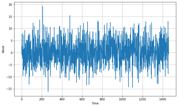

You can find the full time series notebook from Laurence Moroney on Github here.

Train, Validation, and Test Sets

Let's now look at techniques we can use to forecast a given time series.

One way we can do this is with what's called naive forecasting, which takes the last value and assumes that the next value will be the same one. Naive forecasting is typically used for comparison with forecasts generated by more sophisticated techniques.

In order to measure the performance of our forecast we typically split the data into a training period, a validation period, and a test period. This is referred to as fixed partitioning.

If the time series contains seasonality, we want to ensure that each period contains a whole number of seasons (i.e. at least one year if it has annual seasonality).

We then train our model on the training period and evaluate it on the validation period. After tuning the model's hyperparameters to get the desired performance, you can retrain it on the training and validation data, and then test on the unseen test data.

Another way to train and test forecasting models is by starting with a short training period and gradually increasing it over time. This is referred to as roll-forward partitioning.

Metrics to Evaluate Performance

Once we've trained our model we need metrics to evaluate its performance. A few common evaluation metrics include:

• Error: error = forecast - actual
• Mean squared error: mse = np.square(errors).mean()
• Root mean square error: rmse = np.sqrt(mse)
• Mean absolute error: mae = np.abs(errors).mean()
• Mean absolute percentage error: mape = np.abs(errors / x_valid).mean()

Moving Average and Differencing

A common and simple forecasting method is the moving average. To do this, we calculate the average of the values over a fixed period, which is referred to as an averaging window.

A moving average can be useful as it eliminates a lot of noise, although it doesn't anticipate trend or seasonality. For this reason, a moving average can sometimes be worse than a naive forecast.

Differencing is a technique that we can use to avoid this by removing the trend and seasonality of the time series. With differencing, instead of studying the time series itself we study the difference between the value and time $t$ and the value at a previous period, for example 30 days.

We can then use a moving average for forecasting, which gives us a forecast for the differenced time series. After that, we can add back the value of time $t - 30$ days to get the forecast of the original time series.

You can find a notebook on these statistical forecasting techniques from Laurence Moroney on Github here.

Machine Learning Techniques for Time Series Forecasting

Now that we've reviewed statistical techniques for forecasting, let's review several machine learning techniques for forecasting. In addition to building a simple deep neural network for forecasting, we'll look at how we can automate the process of optimizing the learning rate.

Just like other machine learning problems, we first need to divide our data into features and labels. In the case of time series data, our features will be a number a values in the series, and our labels will be the next value.

The number of values that we treat as our feature is referred to as the window size, which means we're using a window of data to train the model in order to predict the next value.

For testing purposes, we can use the tf.data.Dataset class to create a window of time series data for us. For example, we can create a range of 10 values, with a window size of 5, which has been split into 3 batches of shuffled $x$ values and 2 batches of $y$ values below:

dataset = tf.data.Dataset.range(10)
dataset = dataset.window(5, shift=1, drop_remainder=True)
dataset = dataset.flat_map(lambda window: window.batch(5))
dataset = dataset.map(lambda window: (window[:-1], window[-1:]))
dataset = dataset.shuffle(buffer_size=10)
dataset = dataset.batch(2).prefetch(1)
for x,y in dataset:
  print("x = ", x.numpy())
  print("y = ", y.numpy())

Feeding a Windowed Dataset into a Neural Network

Now that we've reviewed how to use tf.data.Datasets to create windows of data, let's look at how to adapt this code in order to feed it into a neural network for training.

We can start with a function called windowed_dataset that takes in a data series and parameters for the window_size, the batch_size to use in training, and the size of the shuffle_buffer that determines how the data will be shuffled. Here's how the function works:

• First we need to create a dataset from the series with tf.data.Dataset
• We then use the window method to split the data based on our window_size
• We then flatten the data to make it easier to work with flat_map
• We then shuffle the data and pass in the shuffle_buffer
• The shuffled data is then split into $x$'s and $y$, which is the last element
• The data is then batched into our batch_size and returned

def windowed_dataset(series, window_size, batch_size, shuffle_buffer):
  dataset = tf.data.Dataset.from_tensor_slices(series)
  dataset = dataset.window(window_size + 1, shift=1, drop_remainder=True)
  dataset = dataset.flat_map(lambda window: window.batch(window_size + 1))
  dataset = dataset.shuffle(shuffle_buffer).map(lambda window: (window[:-1], window[-1]))
  dataset = dataset.batch(batch_size).prefetch(1)
  return dataset

Single Layer Neural Network

Now that we have a windowed dataset we can train a neural network with it. To start, we'll use a single layer neural network thats essentially linear regression. Before training, we need to split our data into training and testing sets as follows:

split_time = 1000
time_train = time[:split_time]
x_train = series[:split_time]
time_valid = time[split_time:]
x_valid = series[split_time:]

Below is the code to do a simple linear regression, which works as follows:

• We start by setting the constants that we want to pass into our windowed_dataset function
• We create our dataset by passing in the synthetic series (introduced in the first section) and the other constants
• We then create a single Dense layer where in the input_shape is the window_size
• We define our model as Sequential that contains our sole layer
• We compile and fit the model with a mse loss function and SGD optimizer

window_size = 20
batch_size = 32
shuffle_buffer_size = 1000

dataset = windowed_dataset(x_train, window_size, batch_size, shuffle_buffer_size)
print(dataset)
l0 = tf.keras.layers.Dense(1, input_shape=[window_size])
model = tf.keras.models.Sequential([l0])

model.compile(loss="mse", optimizer=tf.keras.optimizers.SGD(lr=1e-6, momentum=0.9))
model.fit(dataset,epochs=100,verbose=0)

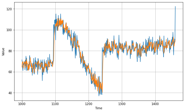
In this case we get a mean absolute error of roughly 5.1. You can find the full notebook for this code from Laurence Moroney on Github here.

Deep Neural Network for Time Series Forecasting

We just looked at using a single layer neural network for time series forecasting, which was effectively linear regression. Now let's see how we can expand on this and create a deep neural network to improve our model accuracy.

The model below is similar to the single layer network, although in this case we're using three layers:

• The layers have 10, 10, and 1 neuron
• The input_shape is still the window_size
• We activate each layer with a relu

model = tf.keras.models.Sequential([
    tf.keras.layers.Dense(10, input_shape=[window_size], activation="relu"), 
    tf.keras.layers.Dense(10, activation="relu"), 
    tf.keras.layers.Dense(1)
])

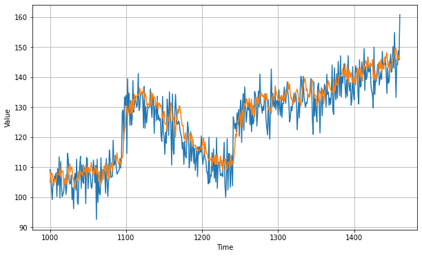
In this case the mean absolute error is 4.9 so the model has improved slightly.

With this model, however, we're still choosing a learning rate randomly. Instead, in order to determine the optimal learning rate we can use tf.keras.callbacks to tweak the learning rate using a LearningRateScheduler:

lr_schedule = tf.keras.callbacks.LearningRateScheduler(
    lambda epoch: 1e-8 * 10**(epoch / 20))

We can then plot the last epoch against the learning rate per epoch:

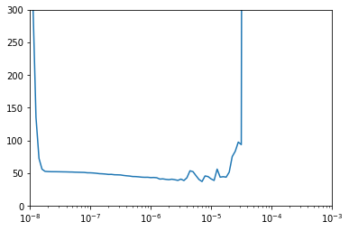
We can then use the lowest point of the curve, which is roughly 8e-6. If we set this as our learning rate and retrain the model on 500 epochs, we can see the mean absolute error improves to 4.7. You can find the code for this example on Laurence Moroney's Github here.

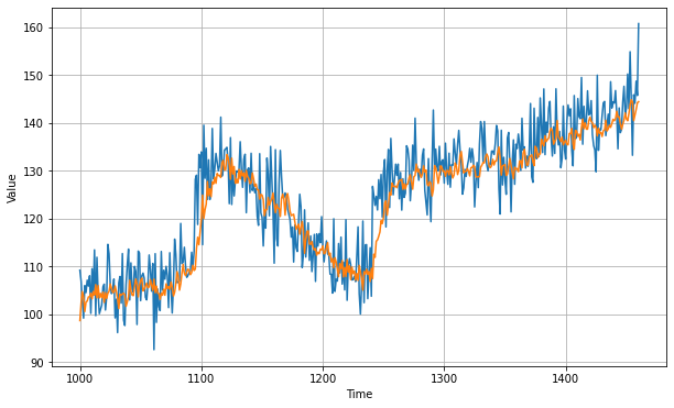
In this example, there's still no sequencing taken into account, although in a time series like this the values immediately before the prediction are more likely to have an impact than those further in the past. One way to apply sequencing is to use a recurrent neural network (RNN) or LSTM.

We won't cover RNNs or LSTMs for time series forecasting in this article, although you can learn about them in Week 3 of this course on Sequences, Time Series, and Prediction.

Summary: Machine Learning for Time Series Forecasting

In this article we introduced several machine learning techniques for time series forecasting. First, we looked at common attributes of time series and how we can generate them synthetically with Python and TensorFlow. We then looked at creating single layer and multi-layer neural networks for time series forecasting.

These techniques covered in this article are relatively rudimentary, so in the next article we'll look at how to use sequencing with RNNs and LSTMs for forecasting.

Resources

• DeepLearning.AI TensorFlow Developer Professional Certificate