This article was originally posted on 2019-04-06 and updated on 2022-11-17.
I. Project Overview
The search for algorithms that can predict future price movements is the holy grail of finance, and has been coined the truth by quants.
While algorithmic trading is nothing new and the computerization of order flow began in the 1970's, the last decade has seen a radical shift in three areas causing what has been termed the fourth industrial revolution.
As this Machine Learning & Big Data paper by J.P. Morgan [1] puts it:
In fact, over the past year, the exponential increase of the amount and types of data available to investors prompted some to completely change their business strategy and adopt a ‘Big Data’ investment framework. Other investors may be unsure on how to assess the relevance of Big Data and Machine Learning, how much to invest in it, and many are still paralyzed in the face of what is also called the ‘Fourth Industrial Revolution’.
In short, massive increases in data, access to low-cost computing power, and advances in machine learning have significantly changed the financial industry. This paper will explore how several machine and deep learning algorithms can be applied in the cryptocurrency market.
This post is part of the capstone project for the Machine Learning Engineer Nanodegree from Udacity.
If you're interested in learning more about machine learning for trading and investing, check out our AI investment research platform, the MLQ app.
The platform combines fundamentals, alternative data, and ML-based insights.
You can learn more about the MLQ app here or sign up for a free account here.
This post may contain affiliate links. See our policy page for more information.
Problem Statement
A common method for price prediction is regression-based strategies. Such strategies use regression analysis to extrapolate a trend to derive a financial instrument's direction of future price movement.
The problem to be solved, then, is understanding the relationship between historical data and future price prediction. In other words, we are looking for the relationship between the dependent and independent variables.
Linear regression is appropriate for this problem as it analyzes two separate variables in order to find a single relationship. To solve this problem, we will first use a linear ordinary least squares (OLS) model and then a neural network regression model using Tensorflow and Keras.
Stay up to date with AI
II. Analysis
In order to implement a data-driven investment approach we first need to obtain and understand our dataset, then we need to preprocess our data and implement the machine learning models, and finally, we need to analyze the results against a benchmark and suggest improvements for the models.
The metric we will be using to analyze each model is the coefficient of determination, or R2, which is: “a statistical measure that represents the proportion of the variance for a dependent variable that's explained by an independent variable.” [2].
The equation for R2 is as follows:
R2 = 1 - (Explained Variation / Total Variation)
I have chosen R2 as it is an important metric in finance that can be used to measure the percentage of the performance of an asset as a result of a benchmark. It is important to note that the R2 does have limitations as it simply provides an estimate of the relationship between price movements, but this does not necessarily indicate when the machine learning model is good or bad or if the predictions are biased.
Benchmark
The benchmark I will use is an R2 score of 0. This number was chosen because financial asset (including cryptocurrencies) returns are often said to be unpredictable. An R2 greater than 0 indicates that there is a relationship between the dependent and independent variable and an R2 less than 0 suggests otherwise.
Datasets & Inputs
The dataset I have chosen to use is the largest cryptocurrency in terms of market capitalization - Bitcoin, relative to the US dollar (BTC-USD). The time frame for the dataset will be from 2016-01-01 to 2018-09-18, and the dataset have been downloaded from Quandl using the Bitfinex source [3].
# import packages
import talib as ta
import pandas as pd
import numpy as np
import matplotlib.pyplot as plt

# machine learning packages
from sklearn.linear_model import LogisticRegression
from sklearn import preprocessing
import tensorflow as tf

# measure results
from sklearn.metrics import r2_score

# read csv dataset
df = pd.read_csv("data/btc-usd.csv")
Exploratory Data Analysis
After importing the data we see this dataset has 8 columns and 964 entries. The dataset is daily time series data with the following features: Date, High, Low, Mid, Last, Bid, Ask, Volume.
I will start by reviewing the daily close price, which is the Last column in the dataset. This feature has a minimum value of $359.16, a maximum of $19,210, a mean of $3869.46, and a median of $1775. Also this dataset does have 3 NaN values, which will need to be dropped in the data preprocessing phase.
df.head()

df.tail()

The following graph displays the 50-day simple moving average with the daily closing price for BTC-USD from 2016-01-01:
# Calculate & display 50 day SMA
df['SMA'] = df['Last'].rolling(50).mean()
df[['Last', 'SMA']].plot(title='BTC-USD Daily Price & 50 Day SMA: 2016-Present',figsize=(10,6))
Daily Percent Changes
Using machine learning in finance can be accomplished in many ways such as predicting the raw prices of our stocks, but as described in this Machine Learning for Finance DataCamp course, typically we will predict percent changes [4]. This makes it easier to create a general-purpose model for stock price prediction.
To get the percent change over a particular time period I have used the pct_change function on a pandas dataframe. The following graph displays a histogram of daily percent changes over time, which we see is right-skewed and has a nearly normal distribution.
# Histogram of the daily price change percent of 'Last' price
df['Last'].pct_change().plot.hist(bins=50)
plt.title('Daily Price: 1-Day Percent Change')
plt.show()
The next step is to shift our pandas dataframe by -5 in order to create a new column with the closing price 5 days in the future, this column is called 5_day-future_close. The 5-day percent changes of the daily price for the current day, and 5 days in the future are then created. After creating these columns, the correlation between our percent price changes (present and future) is calculated to see if previous price changes can predict future price changes. We can see correlation is near 0 at 0.037, which indicates that the two variables are not linearly correlated.
# Create 5-day % changes of Last for the current day, and 5 days in the future
df['5d_future_close'] = df['Last'].shift(-5)
df['5d_close_future_pct'] = df['5d_future_close'].pct_change(5)
df['5d_close_pct'] = df['Last'].pct_change(5)
# Calculate the correlation matrix between the 5d close pecentage changes (current and future)
corr = df[['5d_close_pct', '5d_close_future_pct']].corr()# Scatter the current 5-day percent change vs the future 5-day percent change
plt.scatter(df['5d_close_pct'], df['5d_close_future_pct'])
plt.title('Current vs. Future 5-Day % Change')
plt.show()Algorithms & Techniques
In this section, we will review the algorithms that will be applied to the dataset: in particular, linear regression and a deep learning model.
1. Linear Regression
Linear regression is used to extrapolate a trend from the underlying asset. Linear regression and ordinary least squares (OLS) are decades-old statistical techniques that can be used to extrapolate a trend in the underlying asset and predict the direction of future price movement. A simple example of linear regression trend extrapolation can be seen below from Ch. 5 of Python for Algorithmic Trading [5]:
# generate evenly spaced grid for x values 0-10
x = np.linspace(0, 10)
# generate randomized data for y values
y = x + np.random.standard_normal(len(x))
# calculate OLS regression of degree 1
reg = np.polyfit(x, y, deg=1)
# print optimal parameter values
regarray([ 1.01729281, -0.00614815])
# create new figure object
plt.figure(figsize=(10, 6))

# plot original data as dots
plt.plot(x, y, 'bo', label='data')

# plot regression line
plt.plot(x, np.polyval(reg, x), 'r', lw=2.5, label='linear regression')

# create legend
plt.legend(loc=0)
plt.figure(figsize=(10, 6))
plt.plot(x, y, 'bo', label='data')
# generate an increased number of x values
xn = np.linspace(0, 20)
plt.plot(xn, np.polyval(reg, xn), 'r', lw=2.5, label='linear regression')
plt.legend(loc=0)2. Neural Network Regression
Finally, we will look a neural network regression algorithm to predict the future price of an asset. Loosely modeled after neurons in a biological brain, neural networks are connected by nodes that transmit a signal from one another through what are referred to as hidden layers. The final layer in the neural network is our target prediction variable, which in our case will be a future price prediction. To solve this, this section will make use of the deep learning library Tensorflow with Keras running on top of it.
III. Methodology
Data Preprocessing
Now that we are familiar with our data, it is time to prepare it for machine learning. The first step is to create features and targets. Our features are the inputs we use to predict future price changes with, in this case we are using historical data points as features, and our target is the 5-day future price change.
# a list of the feature names for later
feature_names = ['5d_close_pct']
We want to incorporate historical data as our features, for example, the price changes in the last 50 days. Instead of including each daily price percent changes, we can concentrate historical data into a single point using simple moving averages. A simple moving average (SMA) is the average of a value in the last n days. The features I have created are SMA’s for the time periods of 14, 30, and 50 days.
# Create SMA moving averages and rsi for timeperiods of 14, 30, and 50
for n in [14, 30, 50]:

     # Create the SMA indicator and divide by 'Last'
      df['ma' + str(n)] = ta.SMA(df['Last'].values,
      timeperiod=n) / df['Last']

     # Add SMA to the feature name list
     feature_names = feature_names + ['ma' + str(n)]

print(feature_names)
['5d_close_pct', 'ma14', 'ma30', 'ma50']
# Drop all na values
df = df.dropna()

# Create features and targets
# use feature_names for features; 5d_close_future_pct for targets
features = df[feature_names]
targets = df['5d_close_future_pct']

# Create DataFrame from target column and feature columns
feat_targ_df = df[['5d_close_future_pct'] + feature_names]

# Calculate correlation matrix
corr = feat_targ_df.corr()
print(corr)
The SMA indicator is calculated using the Ta-Lib python package. We can now use these indicators for prediction by creating a DataFrame that includes both a list of our features and the target 5-day future percent change. This is done so that we can analyze if there are correlations between the features and targets before implementing our machine learning algorithms. The following plot uses the seaborn library to visualize a heatmap of the correlations:
import seaborn as sns
# Plot heatmap of correlation matrix
sns.heatmap(corr, annot=True)
plt.yticks(rotation=0); plt.xticks(rotation=90) # fix ticklabel directions
plt.show() # show the plot
Generally, we consider a correlation of 0.2 or greater to signify that there are linear correlations between the variables. From this heatmap, however, we see that none of the variables fit this criteria in relation to our 5-day future price change target.
Algorithm Implementation
Now that we have prepared our data for machine learning, we will start implementing a linear model with our data. To accomplish this we need to split our data in train and test sets - in this case 80% of the data is used for training and 20% for testing.
The purpose of this is to fit our model to the training data and then test on the most recent data to understand how our algorithm will perform on unseen data. A key difference in modeling financial time-series data is that we can’t use sklearn’s train_test_split function because it randomly shuffles the data.
import statsmodels.api as sm

# Add a constant to the features
linear_features = sm.add_constant(features)

# Create a size for the training set that is 80% of the total number of rows
#.shape gives us the number of rows in our data, and convert to an int
train_size = int(0.8 * features.shape[0])

# split features and targets using python indexing
train_features = linear_features[:train_size]
train_targets = targets[:train_size]
test_features = linear_features[train_size:]
test_targets = targets[train_size:]
print(linear_features.shape, train_features.shape, test_features.shape)
(910, 5) (728, 5) (182, 5)
1. Linear model
For linear models, we need to add a constant to our features, which adds a column of 1’s for a y intercept term. To do this we will use statsmodels add_contstant function, and then we will the data into train and test subsets.
Now that we have these two subsets we can fit a linear model by using the Ordinary Least Squares (OLS) function from statsmodels. After fitting the data, the OLS Regression Results are printed and displayed below:
# Create the linear model and complete the least squares fit
model = sm.OLS(train_targets, train_features)
results = model.fit()  # fit the model
print(results.summary())

# examine pvalues
# Features with p <= 0.05 are typically considered significantly different from 0
print(results.pvalues)

# Make predictions from our model for train and test sets
train_predictions = results.predict(train_features)
test_predictions = results.predict(test_features)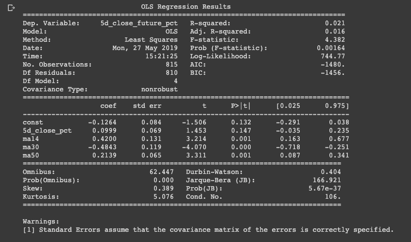
As this displays many results, the one we will focus on is $R2$. An $R2$ of 1 indicates a perfect fit, and the lower the $R2$ value the worse our fit. From the results we see an $R2$ of 0.017, indicating the dependant variable does not explain the independent variable. This is to be expected however, since linear models are one of the simplest machine learning models available.
2. Neural Network
The use of neural networks has rapidly grown due to the exponential increase in GPU computational power over time, the size of data available, and improvements in software. Neural networks are similar to the previous models we have used in that they use features and targets to produce predictions, however neural networks have been shown to outperform other models because they capture variable interactions, have non-linearity, and are highly customizable.
Neural network models typically work better with standardized data, and one way to do this is by scaling our features. To do this we use sklearn’s scale feature, which sets the mean to 0 and standard deviation to 1. A histogram of the scaled data are plotted below:
# Import scale
from sklearn.preprocessing import scale

# Standardize the train and test features
scaled_train_features = scale(train_features)
scaled_test_features = scale(test_features)

# Plot histograms of the features before and after scaling
f, ax = plt.subplots(nrows=2, ncols=1)
train_features.iloc[:, 2].hist(ax=ax[0])
ax[1].hist(scaled_train_features[:,2])
plt.show()
Each layer of our neural network uses input, a weight, a bias and an activation function to add non-linearity. We will use a common activation function called ReLu, or Rectified Linear Units, which is 0 for negative numbers and linear for positive numbers, to add non-linearity.
Predictions are made by passing data through our neural network in the forward direction, and the final node yields the prediction - this is know as forward propagation. Once we have our predictions we use the loss function to compare our predictions and targets. For regression, we often use the mean-squared-error loss function.
We then use our error from the loss function and pass this backwards through the network, which updates weights and biases in order to improve our predictions - this is known as back propagation. Back propagation is how neural networks “learn”, and is part of the reason why we needed to standardize our data earlier.
To implement our neural network we use the Keras library with TensorFlow backend. Keras is a high level API that allows us to build neural networks with minimal code, but still allows for customization. In order to test several different models, I created a model_func function to test different numbers of epochs and layers. I then printed out the loss function of the model with the best R2 score. In the model I used the ReLu activation function and the last layer is 1 node, and has a linear activation function.
After creating the model, we then compile the model with an adam optimizer, and a loss function - in this case mse , or mean squared error. We then fit the model with our features and targets, and specify the number of epochs - or training cycles. After training our model we plot the loss vs. epochs as we want to see that the loss has flattened out.
After this I have calculated the R2 metric and plotted the prediction vs. actual values, which are displayed below:
from keras.models import Sequential
from keras.layers import Dense
epochs =[25, 50, 75, 100]
layers = [[10,20,1], [15,20,1]]

# Create the model
def model_func(layer):
    model_1 = Sequential()
    model_1.add(Dense(layer[0],
        input_dim=scaled_train_features.shape[1], activation='relu'))
    model_1.add(Dense(layer[1], activation='relu'))
    model_1.add(Dense(layer[2], activation='linear'))
    return model_1

# Fit the model
model = 1
final_model = None
max = -100000

for epoch in epochs:
        for layer in layers:
            model_1 = model_func(layer)
            model_1.compile(optimizer='adam', loss='mse')
            history = model_1.fit(scaled_train_features, train_targets, epochs=epoch)
            train_preds = model_1.predict(scaled_train_features)
            print (model, " mean is: ", np.mean(train_preds), " variance is: ", np.var(train_preds)
            if(max < r2_score(train_targets, train_preds))
            max = r2_score(train_targets, train_preds)
            final_model = model_1
        plt.plot(history.history['loss'])
        # Use the last loss as the title
        plt.title('Loss Function: ' + str(round(history.history['loss'][-1], 6)))
        plt.show()
Epoch 25/25 - loss: 0.00941 mean is: 0.027999338 variance is: 0.0007452075
Epoch 50/50 - loss: 0.0086 1 mean is: 0.014622233 variance is: 0.0011360508
Epoch 50/50 - loss: 0.0082 1 mean is: 0.021894086 variance is: 0.0014698462
Epoch 75/75 - loss: 0.0085 1 mean is: 0.023084635 variance is: 0.000825176
Epoch 75/75 - loss: 0.0081 1 mean is: 0.0371084 variance is: 0.0016342839
Epoch 100/100 - loss: 0.0085 1 mean is: 0.030176878 variance is: 0.0014209631
Epoch 100/100 - loss: 0.0079 1 mean is: 0.02349373 variance is: 0.0015530719
IV. Results
In order to validate the neural network model’s robustness, I tested 25, 50, 75, and 100 epochs, as well as [10, 20, 1] and [15, 20, 1] for the number of layers. From these tests I see that 100 epochs with [15, 20, 1] layers has the best loss function at 0.007863. We also see the mean and the variance for this model are 0.0234 and 0.0015 respectively.
# Plot the losses from the fit
plt.plot(history.history['loss'])

# Use the last loss as the title
plt.title('Loss Function: ' + str(round(history.history['loss'][-1], 6)))
plt.show()
from sklearn.metrics import r2_score
# Calculate R^2 score
train_preds = model_1.predict(scaled_train_features)
test_preds = model_1.predict(scaled_test_features)
print(r2_score(train_targets, train_preds))
print(r2_score(test_targets, test_preds))0.23169230829492393
-0.17974375559134725 # Plot predictions vs actual
plt.scatter(train_preds, train_targets)
plt.xlabel('Predictions')
plt.ylabel('Actual')
plt.show()From these tests, we also see that the mean, variance, and loss functions do not change very much for each model. As we can see from these models, the R2 measure is low for all of the models. Since all of these models are relatively simple, however, these results are to be expected. The first step towards improving the models would be adding more features. Other features that could be added include volume, fundamental data, and more engineered technical features using Ta-Lib. Another possible way to improve our neural network model is with custom loss functions.
The final model I have chosen for this project is the neural network. Although it does not have an R2 higher than the benchmark of 0, neural networks have been shown to outperform all other machine learning models and the parameters can be changed to improved performance.
Model Refinement
In order to try and refine the model I will make use of a custom loss function. Since direction is an important aspect of price change prediction, one way to guide our neural network is to apply a penalty to incorrect direction prediction. We can still use the mean squared error (MSE) penalty, but if the direction is wrong we’ll multiply the loss by a penalty factor.
In order to implement custom loss functions we will use the TensorFlow backend again. We then create the loss function as a Python function, which we’re calling mean_squared_error. We pass in y_true, and y_pred as parameters for the actual and predicted values. We then take the difference of actual and predicted values, and square the result with tf.square. Following this, we take the average of that value with tf.reduce_mean across the -1 axis, which is the last axis. We then return that value as the loss.
The next step is to enable to use of our loss value by importing keras.losses. We set this function as part of keras.losses, which makes it available for use in our model. We then fit the model with our MSE loss function. We can now add a penalty for incorrect direction predictions. We first check if the sign of the prediction and the actual value differ. The correct direction is represented by a positive value, and a negative value means the model has chosen the wrong direction.
We now create our custom loss function called sign_penalty and use a penalty value of 10. We then create a conditional statement and return the average of our squared errors, and add our loss function to keras.losses. The results of the first custom loss function are displayed below:
# code inspired by Machine Learning for Finance - DataCamp course [6]
import keras.losses
import tensorflow as tf
# Create loss function
def sign_penalty(y_true, y_pred):
penalty = 100.
loss = tf.where(tf.less(y_true * y_pred, 0), \
penalty * tf.square(y_true - y_pred), \
tf.square(y_true - y_pred))
return tf.reduce_mean(loss, axis=-1)
keras.losses.sign_penalty = sign_penalty # enable use of loss with keras
print(keras.losses.sign_penalty)# Create the model
model_2 = Sequential()
model_2.add(Dense(100, input_dim=scaled_train_features.shape[1], activation='relu'))
model_2.add(Dense(20, activation='relu'))
model_2.add(Dense(1, activation='linear'))
# Fit the model with our custom 'sign_penalty' loss function
model_2.compile(optimizer='adam', loss=sign_penalty)
history = model_2.fit(scaled_train_features, train_targets, epochs=100)
plt.plot(history.history['loss'])
plt.title('loss:' + str(round(history.history['loss'][-1], 6)))
plt.show() Epoch 100/100 - loss: 0.2637
Conclusion
To summarize this project: we started with the problem of single asset price prediction based on historical data. Several features of the data were visualized to understand it better and then the data was preprocessed for machine learning. We then implemented two different machine learning models: OLS linear regression and a neural network model with Keras and TensorFlow. The R2 metric for each model was recorded, which provides a starting point for improving the models in the future. The goal of this paper was not necessarily to find a model that will outperform the markets, but rather to research how regression-based machine learning models can be applied to the financial markets. The possible ways to improve the models include adding more features, and creating a custom loss function for the neural network.
For the final model, we can see that the loss function actually got worse by introducing a custom loss function. The following is the R2 score and a scatter plot of the custom loss neural network model:
# Evaluate R^2 scores
train_preds = model_2.predict(scaled_train_features)
test_preds = model_2.predict(scaled_test_features)
print(r2_score(train_targets, train_preds))
print(r2_score(test_targets, test_preds))

# Scatter the predictions vs actual
plt.scatter(train_preds, train_targets, label='train', color='blue')
plt.scatter(test_preds, test_targets, label='test', color='red')  # plot test set
plt.xlabel('Predictions')
plt.ylabel('Actual')
plt.legend(); plt.show()
0.009378061381353886
0.022762820123008676 As we can see the did not get better with the custom loss function better and the R2 metric is roughly the same. Further improvements to our model could be changing the type of neural network algorithm used. In this case I used a regression algorithm, although techniques that I researched and would consider using are Deep Reinforcement Learning.
This type of neural network uses a state-action-reward function and have become increasingly popular recently. If you want to learn more about Deep Reinforcement Learning for Trading you can read this guide on the subject.

