Introduction to Generative Adversarial Networks (GANs): Intuition & Theory

Generative Adversarial Networks, or GANs, are an emergent class of deep learning that have been used for everything from creating deep fakes, synthetic data, creating NFT art, and much more.

In this article, we'll introduce the theory and intuition of generative models and GANs. This article is based on notes from the first course in the Generative Adversarial Networks (GANs) Specialization from deeplearning.ai and is organized as follows:

• Introduction to Generative Models
• Real-World Applications of GANs
• Intuition of GANs
• The Discriminator
• The Generator
• BCE Cost Function

This post may contain affiliate links. See our policy page for more information.

Introduction to Generative Models

In this section, we'll discuss the intuition and theory behind generative models, of which GANs are a part of. Below is a summary of the differences between generative vs. discriminative models.

Discriminative Models

• Discriminative models are typically used for classification in machine learning
• Discriminative models take a set of features $X$ and determine a category or class $Y$, $X \rightarrow Y$
• Discriminative models try and model the probability of class $Y$ given a set of features $X$, $P(Y|X)$

Generative Models

• Generative models attempt to create a realistic representation of a class, for example a realistic image of a cat
• Generative models take input in the form of noise $\xi$, which are random values going into the model
• The generative model may also take in a class $Y$, such as a cats, dogs, and so on
• From these inputs, the goal of the model is to generate a set of features $X$ that look like a realistic image of a cat
• $\xi, Y \rightarrow X$

More generally, generative models try and capture the probability distribution of $X$ given a class $Y$, or $P(X|Y)$

With the addition of random inputs, or noise, a generative model can create a realistic yet diverse set of representations of class $Y$.

Two of the most popular generative models include Variational Autoencoders (VAEs) and Generative Adversarial Networks (GANs), below is a brief summary of each.

Variational Autoencoders

• Variational autoencoders work with two models—an encoder and a decoder—which are typically neural networks
• The model learns by feeding in realistic images into the encoder
• The decoders job is to determine how to represent the image in latent space
• In other words, the decoders goal is to reconstruct a realistic image from the encoder

You can learn more about variational autoencoders in the article below:

Generative Modeling: What is a Variational Autoencoder (VAE)?

Variational autoencoders combine techniques from deep learning and Bayesian machine learning, specifically variational inference.

MLQPeter Foy

Generative Adversarial Networks

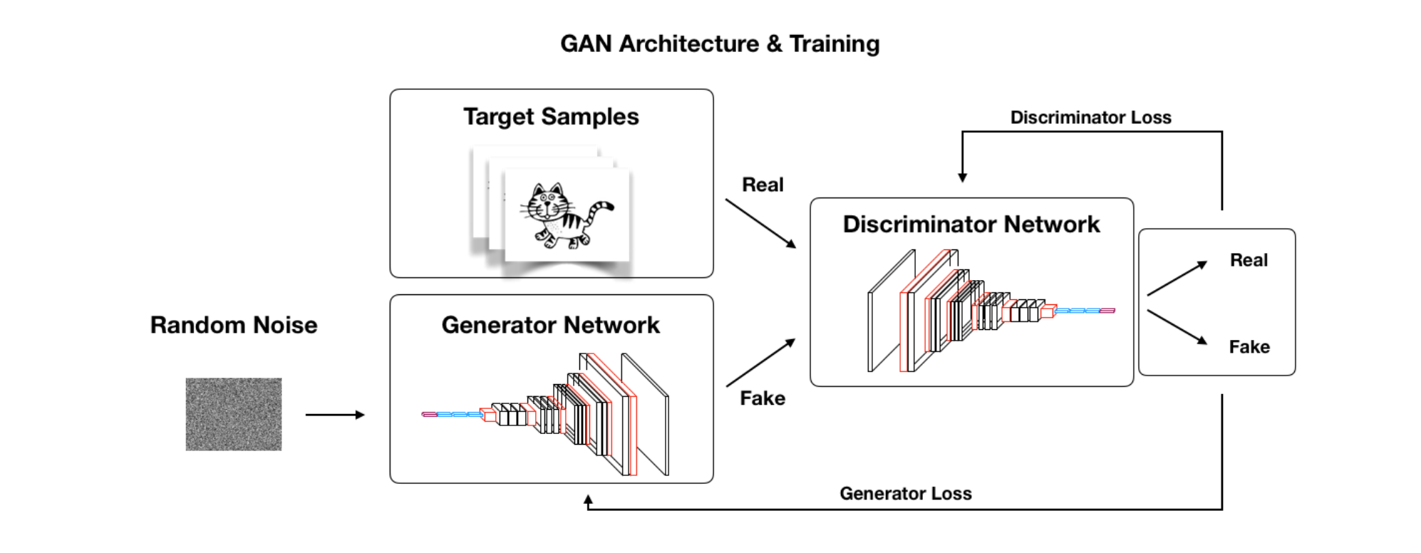
• GANs are composed of two models—a generator and a discriminator
• The generator takes in some random noise as input and attempts to output a realistic image of a cat, for example
• In some sense, the generators role is similar to a decoder in VAEs, although is there is no guiding encoder that determines what the noise vector should look like
• Instead, the discriminator is looking at fake and real images and trying to determine which are real or not
• Over time, each model tries to improve by "competing" with each other, hence the name adversarial
• After training, the generator should be able to take in any random noise and produce a realistic image

Real-World Applications of GANs

Now that we have a high-level overview of generative models, let's look at a few real-world applications of GANs.

Below is a tweet from the creator of GANs, Ian Goodfellow, that highlights the progress they have made in the field of face generation from 2014 to 2018:

Since then, GANs have continued to improve significantly. Also, keep in mind that GANs are not limited to generating images. In the context of quantitative finance, for example, an interesting application is the field of synthetic data generation.

You can learn more GANs for synthetic data in the article below:

Synthetic Financial Data with Generative Adversarial Networks (GANs)

In order to overcome the limitations of data scarcity, privacy, and costs, GANs for generating synthetic financial data may be essential in the adoption of AI.

MLQPeter Foy

A few other applications of GANs include:

• Image translation, or taking an image from one domain and translating it to another, for example changing an image of a horse into a zebra
• Image animation, or taking a still image and turning it into an animation
• Generative design, for example generating 3D images of furniture, medical data, and much more

There are also several companies using GANs in interesting ways, including:

• Adobe is looking at ways to use GANs to create a next generation photoshop
• Google is using GANs for text generation
• IBM is using GANs for data augmentation
• Snapchat and TikTok are using GANs to create image filters
• Disney and Pixar are using GANs for to create high-resolution content

Intuition of GANs

As mentioned, a GAN learns by having the generator and discriminator compete against each other. In this section, we'll discuss the goals of each competing model and how that results in the generator being able to produce realistic samples.

The generator and discriminator are typically two different neural networks. The generators learns to generate fake samples in an attempt to fool the discriminator. The discriminator learns how to distinguish between what's fake and what's real.

As an analogy, you can think of the generator as someone trying to forge a painting and the discriminator as the art inspector.

In order to start this competition, you need a collection of real images, for example the original paintings. In the beginning, the generator has no idea how to produce realistic representations.

The generator also isn't allowed to see any of the real images, it has no idea what it's trying to replicate in the beginning.

On the discriminator side, in the beginning it also doesn't know for sure what's fake or real. To start the competition, we first need to train the discriminator using real artwork so it knows what's real and what's fake.

As the discriminator is learning, we tell it which ones are fake vs. real so it knows whether it's right or wrong in distinguishing between the two classes. As it receives more and more images, the discriminator should improve at distinguishing between the two.

As the generator starts producing images, it will then use the scores provided by the generator that tell it how close it is to the real thing. For example, the discriminator might say one image is 5% real, another is 20% real, and so on.

With this information, the generator continues to learn and tries to get closer and closer to a realistic representation.

In summary:

• The generator's goal is to fool the discriminator
• The discriminators goals to distinguish between real and fake
• Each model learns by competing with each other
• After training, the fake images should look realistic

Next, we'll take this intuition and discuss how the competition works in more detail.

The Discriminator

The discriminator model is a type of classifier that distinguishes between classes.

One type of model for a classifier is a neural network that takes in features $X$ as input. For example, it will take $X_0$, $X_1$...$X_n$ for $n$ different features.

It then computes a series of nonlinearities and outputs a probability for a set of categories.

In the beginning, it will not be very good at distinguishing between classes and improves over time as it learns from the real or fake labels.

This learning process can be summarized as follows:

• We have input features $X$ and a set of labels $Y$ for each class
• The neural network takes in the features an learns a set of parameters, or $\theta$
• The weights in the neural network change over time as the model learns what a cat, dog, and bird look like, for example
• The parameter data are trying to map the features $X$ to class $Y$
• The predictions, or $\hat{Y}$, aren't labels, but are trying to get as close to $Y$ as possible
• In other words, the goal is to minimize the difference between the true value of $Y$ and the prediction value $\hat{Y}$— this is the goal of the cost function
• From this cost function, we can update the parameters $\theta$ to get $\hat{Y}$ closer and closer to $Y$

We then repeat this process over and over again until it the generator is able to produce realistic representations of whatever we're trying to recreate.

We can describe the goal of the discriminator as trying to model the probability of each class, which we can write mathematically as $P(Y|X)$.

This is a conditional probability distribution as it's prediction the probability of class $Y$ conditioned on certain set of features.

The Generator

The generator's ultimate goal is to produce examples from a certain class.

If you train the model on a set of cat images, the generator will learn how to output a representation of a cat. Every output will also ideally be different each time.

To ensure each output is unique, we input a different set of random vales, which is known as a noise vector.

The noise vector is just a set of a different values, which are fed as input with the class $Y$ into the generators neural network.

This means the features $X_0$, $X_1$...$X_n$ include the class and the numbers in the noise vector.

The generator will then compute a series of nonlinearities from these inputs and return variables that look like a cat.

The generator improves over time in the following way:

• A noise vector $\xi$ is passed into the generator neural network to produce a set of features that attempt to represent an image of a cat, or $\hat{X}$
• The generated image $\hat{X}$ is fed into the discriminator which determines how real or fake it think it is, or $\hat{Y_d}$
• The discriminators prediction $\hat{Y_d}$ is then used to compute a cost function $\hat{Y}$ that essentially looks at how far the generated image is from being considered real by the discriminator
• The generator wants $\hat{Y_d}$ to be as close to 1, or real, as possible and the discriminator wants it to be 0, meaning it knows its fake
• The generator uses the cost function $\hat{Y}$, or the difference between the two, to update its parameters $\theta$, which helps it improve over time

Once we have a generator that is producing realistic representations, we can save the parameters $\theta$ so it can then be sampled from later on.

In this example, the generator is trying to model the features of a cat given the class $Y$, or $P(X|Y)$.

If we only have one class, we don't need to worry about $Y$ and it's just $P(X)$, although it we're modeling multiple classes we need it.

In this case, $P(X)$ is trying to approximate the real distribution of possible cats. This means that more common species or features of cats will have more chances of being generated.

BCE Cost Function

The binary cross-entropy (BCE) cost function is commonly used for training GANs.

Since it's binary, it is well suited to the classification task of determining if a sample is real or fake.

The BCE cost function equation is shown below:

$$J(\theta) = -\frac{1}{m}\sum^m_{i=1}[y^{(i)} log h(x^{(i)}, \theta) + (1 - y^{(i)}) log(1 - h(x^{(i)}, \theta))]$$

Here is a breakdown of the intuition behind this equation:

• The first part $-\frac{1}{m}\sum^m_{i=1}$ refers to the average loss, or average cost, of the whole batch
• $h$ denotes the predictions made by the model
• $y$ is the true label of the different examples
• $x$ are the features that is passed in through the predictions
• $\theta$ are the parameters of whatever is computing the predictions, which in this is case the discriminator
• In the brackets, the first term $y^{(i)} log h(x^{(i)}, \theta)$ is the product of the true label $y$ times the log of the prediction. This term is relevant when the label is 1—it makes it 0 if it is good, or close to 1, and makes it negative infinity if it is bad, or close to 0.
• The second term (1 - y^{(i)}) log(1 - h(x^{(i)}, \theta)) is similar - if the label is 1, it will evaluate to 0. If the label is 0, i.e. fake, and the prediction is close to 1, it will evaluate to negative infinity.

Each of these two terms evaluates to negative infinity if the relevant label of the prediction is close 0, in other words if it is very bad.

This is why there is a negative sign in front of the whole equation—if either term evaluates to a large number in the negative direction, it will then be made to positive infinity. This is useful, since for our cost function what we want is a high value to be bad, and the neural network will try to minimize this value over time.

In summary:

• The BCE cost function has two parts, one that is relevant for each class (real or fake)
• When the prediction and label are similar the BCE cost function is close to zero
• The BCE cost function approaches infinity when the label and prediction are different

Summary: Intuition and Theory of GANs

In a basic GAN, the generator takes in noise $\xi$ and produces fake samples $\hat{X}$.

The generated samples $\hat{X}$ along with real samples $X$ are fed into the discriminator, which then outputs a probability that the sample is real or fake $\hat{Y}$.

The goal of the discriminator is to distinguish between generated examples and real examples. The goal of the generator is to fool the discriminator by produce fake examples that look as real as possible.

In order to train a GAN, we alternate between training the generator and discriminator. The parameters of the discriminator are updated by comparing the predictions and the real labels. By computing the BCE cost function, the gradient is backpropagated and the parameters of the generated are updated.

By training in the alternating fashion, each model should improve together over time at a similar level of skill. The reason for this is that the discriminator has a much easier job, and a common issue is have a discriminator that is much superior than the generator. If the discriminator says a sample is 100% fake, for example. this doesn't help the generator learn where it should grow and learn.

The takeaway is that in training in this alternating fashion, we need to keep the scale of the generator and discriminator close to each other to ensure an effective training process.

Resources

• Generative Adversarial Networks (GANs) Specialization