Deep Reinforcement Learning for Trading: Strategy Development & AutoML

In this guide, we're going to review how deep reinforcement learning can be used to improve the efficiency and performance of existing trading strategies.

The application of deep reinforcement learning for trading has been of great interest for many professionals in finance, although it still remains largely unexplored in terms of practical applications.

That said, reinforcement learning has shown such promise in other fields such as playing the game of Go, playing Starcraft, self-driving cars, improving energy efficiency, and more.

In fact, many AI experts agree that deep reinforcement learning is likely to be the best path towards AGI, or artificial general intelligence, as OpenAI says:

At OpenAI, we believe that deep learning generally—and deep reinforcement learning specifically—will play central roles in the development of powerful AI technology.

If these early advances in reinforcement learning and the predictions of many experts are at least somewhat accurate, it's likely that it will become increasingly important in the field of algorithmic.

This guide is based on notes from reinforcement learning for trading course and is organized as follows:

1. Review of Reinforcement Learning
2. Review of Reinforcement Learning for Trading
3. Q-Networks
4. Policy Gradients
5. LSTMs
6. Applying Neural Networks to Reinforcement Learning
7. Developing a Deep Reinforcement Learning Trading Strategy
8. Review of AutoML

1. Review of Reinforcement Learning

We won't cover the mathematical details of reinforcement learning in this article as we've covered it extensively before, although if you want to learn more check out these articles:

• What is Reinforcement Learning? A Complete Guide for Beginners
• Guide to Deep Reinforcement Learning: Key Concepts & Use Cases
• Deep Reinforcement Learning: Twin Delayed DDPG Algorithm
• Deep Reinforcement Learning: Guide to Deep Q-Learning
• Deep Reinforcement Learning for Trading with TensorFlow 2.0

Reinforcement learning is a branch of machine learning that is based on training an agent how to operate in an environment based on a system of rewards. For example, if you're training an agent how to play a video game it would learn how to operate in the environment by the points earned or lost.

In the context of trading, an agent would learn how to optimize a portfolio based on metrics like profit, loss, volatility, and so on.

A few other key concepts in reinforcement learning include:

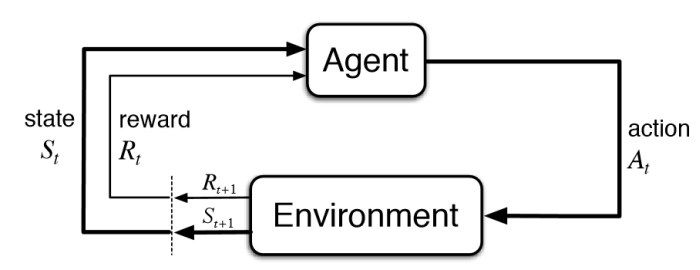
• Agent: This is our AI that we train to interact within the environment
• Environment: This can be anything that gives us an observable state
• State: This is the current position of the agent
• Action: Based on the state, the agent determines the optimal action to take
• Reward: The environment returns a reward, which can be positive or negative

The diagram below from Sutton & Barto's textbook Reinforcement Learning: An Introduction gives you an overview of the reinforcement learning process:

These terms are purposely vague since each of these concepts will mean something different given the task and environment at hand. In the context of trading however, here's what they mean:

• The agent is the trader
• The environment is the market
• The state relates to statistics about the current market, which could be a number of different things like daily moving averages, high of day, volume, etc.
• The actions could include going long, short, closing a position, or choosing a particular asset for a portfolio
• The reward could be profit, loss, volatility, Sharpe Ratio, or any other performance metric

A key point about reinforcement learning for trading is that the agent won't give us predictions like price target, sentiment, and so on.

Instead, the agent will take the predictions from other machine learning or statistical models and decide what the optimal actions are to maximize the cumulative expected reward.

A Brief History of Reinforcement Learning

Before we get into reinforcement learning for trading, let's briefly review the history of reinforcement learning.

The practice of reinforcement learning has been around for more than 50 years and many of the early technique still influence the development of modern algorithms, these include:

• Value iteration
• Policy iteration
• TD-Lambda
• Q-learning

The start of reinforcement learning goes back to 1957 when Richard Bellman introduced the Bellman equation, which is the basis of the aforementioned algorithms.

To understand the Bellman equation, let's first look at solving the Frozen Lake environment in OpenAI Gym.

Value Iteration

To solve this grid-world problem we're going to use a Markov Decision Process, (MDP), which is a discrete time stochastic control process. In essence, Bellman's approach was to reduce the problem to its simplest possible state and use recursion to solve larger problems.

The Bellman equation works as follows:

$$V(s) = R(s,a) + \gamma (Vs')$$

where:

• $V(s)$ is the value of the current state
• $R(s,a)$ are the rewards received
• and $\gamma (Vs')$ is the discounted future state

The Bellman equation allows us to find a numeric value $V$ for the current state $s$, which is defined as the reward we receive $R$ given the action we take $a$ in state $s$.

We then add that reward to the discounted value $\gamma$ of the new state we end up in $s'$.

The discount factor is between 0 and 1 and can be thought of as a similar concept to the time value of money.

In the context of reinforcement learning, changing the discount factor will change how the agent prioritizes short term vs. long term rewards.

If we have multiple possible actions, we choose our action with what's referred to as the policy function.

This is where to the learning comes in as the goal of our agent is to find a policy function that takes state information and returns the best possible action to take.

There are several strategies for determining the policy function, but for now, we'll just follow the highest value action, which is used referred to as the locally optimal policy, or $\pi*$.

Now we're going to modify the Bellman equation as follows:

$$V^{\pi*}(s) = max_a{R(s,a) + \gamma V^{\pi*}(s')}$$

Here we update the value of the current state with the reward plus the highest-value state we can reach given our current state. As we iterate through actions in the environment we get an optimal policy map.

Policy Iteration

The next breakthrough in reinforcement learning came from the idea of policy iteration.

While value iteration is a powerful way to solve MDPs, it was not the most computationally efficient approach.

Here are the key difference between value iteration and policy iteration from StackOverflow:

• Policy iteration includes: policy evaluation + policy improvement, and the two are repeated iteratively until policy converges.
• Value iteration includes: finding optimal value function + one policy extraction. There is no repeat of the two because once the value function is optimal, then the policy out of it should also be optimal (i.e. converged).

Here is how we update the Bellman equation to include policy iteration:

$$V^{\pi*}(s) = max_a{R(s,a) + \gamma \sum_{s'}P(s'|s,a) V^{\pi*}(s')}$$

Now when we update the value of the state it will be a weighted average of the value of all the next state $s'$ we could end up in.

In practice, policy iteration often converges more quickly than value iteration.

The success of policy iteration brought about two schools of RL thought:

• One way is to focus our effort on estimating the value of our state
• The other way is to focus on finding the policy directly

In short, value iteration is mathematically precise so it takes longer to find an accurate answer. Policy iteration, on the other hand, takes a statistical approach to solve the problem.

TD Learning

While value and policy iteration work well in theory, in practice there aren't that many real-world applications of the techniques.

One of the main challenges of these techniques is figuring out what to do in uncertain situations. In the Frozen Lake environment, we can see the entire environment—the layout, rewards, etc.—but in reality we may have not have any of this information.

Temporal difference learning, or TD-learning, attempts to solve this with what Richard Sutton calls online learning.

Here is the equation for the tabular TD(0) method, which is one of the simplest TD methods:

$$V(s_{t-1}) = V(s_{t-1}) + \alpha_t (R(s_{t-1}, a) + \gamma V(s) - V(s_{t-1}))$$

Here we introduce a new variable $\alpha$ to represent the learning rate.

Now every time the agent takes a time step, it looks at the state it's leaving and alters it based on the new state and any rewards it picked up.

With TD(0) we only update the previous state with the new information, and TD(1) looks across the entire episode. If we add another variable $\lambda$ we can combine these two algorithms into one.

Q-Learning

Q-learning is a popular application of TD(0), which uses a Q-table. Instead of finding the value for a state, Q-learning assigns values to a combination of state and action, so a Q-table uses rows to represent states and columns to represent actions.

Here is a helpful visualization to understand Q-tables from TowardsDataScience:

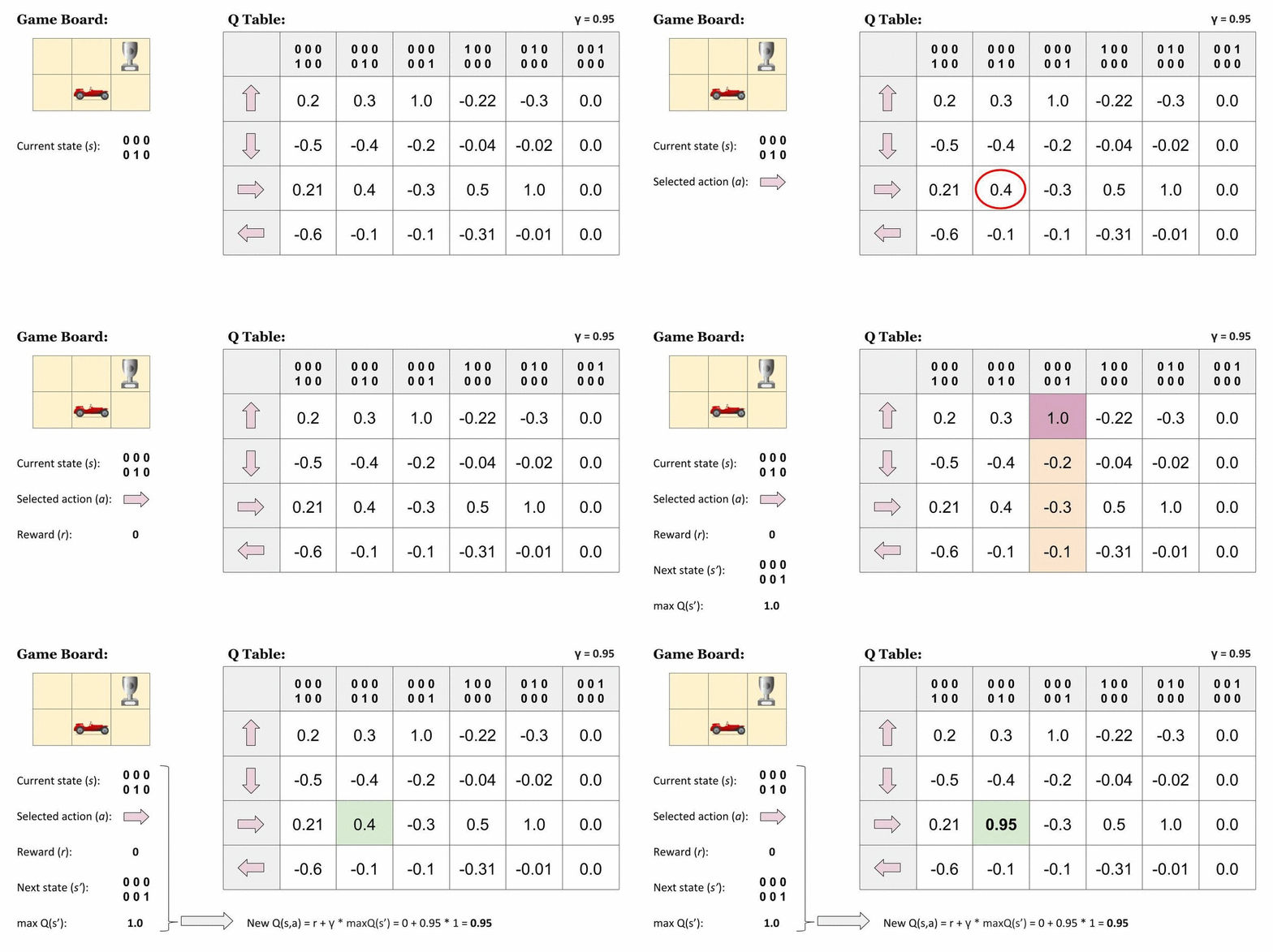
Our policy is going to be taking the maximum value action given the state we're currently in.

Here is the equation for deep Q-learning:

$$Q(s_t,a_t)= Q(s,a)+ _t(r_t + \gamma \cdot max_a{Q(s_{t+1}, a)} - Q(s_t, a_t))$$

We won't cover the full intuition of deep Q-learning in this article, but if you want to learn more check out our Guide to Deep Q-Learning here.

2. Review of Reinforcement Learning for Trading

Now that we've reviewed a few of the core concepts of reinforcement learning, let's review some of the fundamentals of its application to trading.

In particular, we'll look at how we can combine deep learning with reinforcement learning and apply it to a trading strategy.

To recap, deep reinforcement learning puts an agent into a new environment where it learns to take the best decisions based on the circumstances of each state it encounters.

The goal of the agent is to collect information about the environment in order to make an informed decision. It does this by testing how it's actions influence its own rewards in the environment.

The more frequently the agent interacts with the environment, the faster it learns how to maximize its expected rewards.

The main difference between deep reinforcement and other types of machine learning algorithms is that the DRL agents are given a high degree of freedom when it comes to the learning process.

In practice, reinforcement learning for trading involves the following main factors:

• Agent: This is the trader that has access to a brokerage account and periodically checks the market conditions and makes trading decisions
• Environment: The market provides feedback in the form of profit and loss
• State: The state of the environment is not known to the agent—meaning it doesn't know the number of other agents, their actions, their positions, or their orders
• Reward: A naive approach to the reward function would be driven by the absolute maximization of profits, although since that could lead to high risk trading you can use other performance metrics such as the Sharpe ratio

DRL for Trading Strategy Efficiency & Performance

An interesting paper from JP Morgan called Idiosyncrasies and challenges of data driven learning in electronic trading found that a medium frequency electronic trading algorithm will make 3600 decisions each hour, or a decision every second.

This is due to the fact that each action is a consequence of "child orders" of things like price, order type, size, and so on. Here is what they say in the paper:

For electronic trading, an action is a collection of child orders: it consists of multiple concurrent orders with different characteristics: price, size, order type etc. For example, one action can simultaneously be submitting a passive buy order and an aggressive buy order. The passive child order will rest in the order book at the price specified and thus provide liquidity to other market participants. Providing liquidity might eventually be rewarded at the time of trade by locally capturing the spread: trading at a better price vs someone who makes the same trade by taking liquidity. The aggressive child order, on the other hand, can be sent out to capture an opportunity as anticipating a price move. Both form one action. The resulting action space is massively large and increases exponentially with the number of combinations of characteristics we want to use at a moment in time.

What this means is that financial markets are simply too complex for non learning-based algorithms, as the action space is continuously expanding each second.

Existing algorithmic trading models are generally built with two main components: strategy and execution.

In many cases, it will be the trader who determines the strategy and an algorithm handles the execution.

With deep reinforcement learning, however, we're getting closer to a fully autonomous solution that handles both the strategy and execution fo trading.

3. Q-Networks

In this section let's review how neural networks can be applied to reinforcement learning. In particular, we'll look at:

• TD-Gamman
• Deep Q-Networks
• How the loss function is used in deep Q Learning
• The Actor-Critic model vs. deep Q-Networks
• Applying LSTMs to time series data

TD-Gamman

TD-Gammon is one of the first successful reinforcement learning algorithms to use neural networks. It's also one of the first RL algorithms to beat complex strategy games like chess and then backgammon.

One of the reasons TD-Gammon was successful using neural networks instead of simply a Q-table is that a table isn't practical for games like backgammon, whose number of possible game states number in the quintillions.

Another issue with a Q-table is that each state requires a discrete number with a table, although if we have a problem with continuous values we would need to convert it into an integer value.

Instead of trying to account for each possible state position, the author fed in state information to a neural network, which was designed to approximate TD Lambda.

Although TD-Gammon didn't end up actually beat the top backgammon players, the performance was strong enough to warrant testing other neural network based strategies to reinforcement learning.

Deep Q Networks

The next major advancement in applying neural networks to reinforcement took over two decades.

The next big breakthrough was DeepMind's seminal paper in 2013 called Playing Atari with Deep Reinforcement, which used a convolutional neural network with a variant of Q-learning.

Similar to TD-Gammon, it works by feeding state information into the network, and in this case, they fed in pixels on a screen.

Loss Function

There are a few key insights that helped the agent excel in the Atari environment, the first of which is the loss function.

In this case, we still use the Q update function from Q-learning, except instead of it updating a Q-table cell we use it to directly update the weights in our network.

Our new Q-function takes in three parameters: state, action, and the weights of the network.

The final layer of our network has a node for each action and estimates the Q-values of each of the actions given the current state.

The result of this function is the label we're trying to predict.

Memory

The other key insight DeepMind had is called experience replay.

Instead of training after each time step like in TD Learning, we first collect the state transition in a memory buffer. As soon as we've collected enough memories, we pull out a sample batch to train on.

In practice, at each time step we get a bunch of information to train with. We add this information to a memory buffer, which is just a table that we append with a row each time step. To recap, each cycle returns:

• 1 State
• 1 Chosen Action
• 1 Reward
• 1 State Prime

In Python, the buffer is usually a deque, so when the buffer is full older transitions are dropped out, similar to how older memories are forgotten.

4. Policy Gradients

We just reviewed deep Q-learning, which focuses on estimating state action pairs.

Now let's look at another school of reinforcement learning, which focuses on estimating the policy directly.

With deep Q-learning, we built a network that takes in state properties and predicts the value of each action.

Policy gradient based algorithms take in state properties and returns the probability that we should take an action, given our current state.

The policy gradients loss function is as follows:

$$\Delta w = \nabla \pi_w(a^*, s)$$

Actor Critic

Actor Critic is a variant of policy gradient that instead of using vanilla TD1, we bring back the Q-function.

We can use the Q-function to implement a popular version of the algorithm called Advantage Actor Critic (A2C). Another version of the algorithm we can use is called Asynchronous Advantage Actor Critic (A3C).

The Q-function can be broken down into two functions:

• The value function $V$ from TD-Lambda, which estimates the value based on the state
• The advantage function $A$ is how much value a state changes given an action $a$

$$Q(s,a) = V(s) + A(s,a)$$

There are now three sets of output nodes:

• Predict: this tells us the probability we should choose an action
• Actor: this is the same as our policy network from policy gradient
• Critic: this tries to represent the $V$ in our Q-function

To recap, our learning function combines both our Q-function and our policy gradient learning.

5. LSTMs

In this section we're going to look at LSTMs, a type of recurrent neural network that has become increasingly popular in recent years.

First, a sequence model differs from other structured data problems as order the data matters, for example the order of words in a sentence is very important for it to make sense.

While we can use classic deep neural networks for sequence models, recurrent neural networks have usually proved to be better suited for the task.

The logic of an RNN allows it to provide temporal context, meaning if a price of information was shared a few time steps earlier, the hidden state of the network can still use that knowledge to predict the next time step.

While RNNs are useful for sequential modelling, there are two main problems —both of which are related to the gradient: gradients exploding and gradients vanishing.

As gradients pass through the whole sequence, they can be unstable each way, either exploding to large values or vanishing towards zero.

LSTMs, or long short-term memory networks can mitigate these two issues in the following way:

• A generic simple RNN has an input, hidden state that is fed back to the network, and an output that can in some cases be the hidden state itself
• LSTMs improve this simple layout first with a memory cell value that's carried over time
• The gates that influence the memory cell include the forget gate and the input gate, which uses a sigmoid and the tanh function to decide what to keep in memory
• The output gate controls the extent to which the value in the cell is used to compute the output activation of the LSTM unit

Applying LSTMs to Time Series Data

Time series data is a ubiquitous and special type of sequence which we can apply LSTMs to.

If we wanted to use a classic supervised machine learning model, such as a regression model, it can be non-trivial to exactly define our features as well as our target label.

Our target label is future values, but we know to know exactly how long of a period we're predicting.

If you want to learn more about applying LSTMs to time series data, check out this tutorial from Machine Learning Mastery.

7. Developing a Deep Reinforcement Learning Trading Strategy

Now that we have an understanding of the foundations of deep reinforcement learning, let's look at how to use it to develop a trading strategy.

An RL trading strategy is similar to other quantitative systems — it receives data of the current market and acts on by either placing a trade or not. These signals can either go through approval of a human trader, or act 100% autonomously.

As the system trades, the new market state along with order performance is passed to the policy optimization algorithm, and then the revised policy along with new market data is once again analyzed, tested, and passed to the RL trader.

Steps Required to Develop a DRL Trading Strategy

The steps required for deep reinforcement learning algorithm development are as follows:

1. Select the instrument(s) you want to trade
2. Model trading costs and other potential drags on performance, such as slippage
3. Obtain and clean historical data
4. Create an ensemble of algorithms and experiment with inputs
5. Define the action space and decide on a training method
6. Train and backtest the RL trader
7. Go live and deploy the model or retrain it with different parameters

Final Checks Before Going Live With the DRL Strategy

Before going live with the trading strategy, it's recommended to take the following steps:

• Ensure the RL trader performs well for a long enough period of time and in different market conditions
• Ensure the RL trader can perform well on securities or assets that it hasn't been trained on
• The algorithm should have decent performance in the test set, as well as in training and development sets

One way to try and improve the algorithm if it seems to be overfitting is to increase the dropout rate, for the following reasons:

• As a neural network learning, neuron weights settle into their context within the network
• If the neurons are dropped this results in the network learning multiple independent representations.
• As the network becomes less sensitive to the specific weights of neurons it is often better able to generalize and not overfit the data.

8. AutoML

As mentioned, an RL trading strategy doesn't make the actual predictions for things like price prediction or sentiment, instead it takes these inputs and chooses an optimal action.

This means that we still need to develop the machine learning models for prediction, and one of the simpler ways we can do this is with Google Cloud's AutoML.

AutoML is a service that allows you to train high-quality custom machine learning models with minimal effort and machine learning expertise.

Here's how they describe the service:

Cloud AutoML is a suite of machine learning products that enables developers with limited machine learning expertise to train high-quality models specific to their business needs. It relies on Google’s state-of-the-art transfer learning and neural architecture search technology.

AutoML fits into suite of GCP products as follows:

• You can build a custom model, which is time consuming and requires ML expertise
• You can use a pre-trained model, although the downside of these is that the predictions are only good when you're dealing with common data such as social media images or customer reviews
• AutoML sits between these two — a model is trained on your data specifically, but you don't need to write any code to train it

Cloud AutoML follows a standard procedure of three phases:

• Training: You first need to prepare a data set to be used in the supervised training process and then test and evaluate it on unseen data
• Deploying: In this phase we deploy and manage the model, which means we get rid of old or unused models
• Serving: Finally we host the model on a service where it can be used to predict and classify new data

Since traditional machine learning models were relatively hard to create, there was a tendency to ty and make the data set and model all inclusive.

With Cloud AutoML, you can create smaller, more specialized custom models and use them programmatically.

AutoML Vision

AutoML Vision is a cloud product that specializes in training classification models for image data.

The image data needs to be converted to base 64 encoding, which stores the image as a text file.

For model performance it's recommended to remove low frequency labels, since you want 100 times more images with the most common label than the least common.

AutoML NLP

AutoML NLP specializes in training models for text data.

You can upload documents up to 128 kilobytes and can have anywhere from 2-100 labels.

The model is evaluated on average precision, which is the area under the precision/recall curve.

AutoML Tables

AutoML Tables is specialized in tabular data, so while AutoML Vision and NLP are for unstructured data, Tables is for structured data.

The easiest way to import data into AutoML Tables is through BigQuery, although you can also use CSV files.

The data must have between a thousand a hundred million rows, two and a thousand columns, and be a hundred gigabytes or less in size.

To summarize, AutoML allows you to build powerful machine learning models that are customized to your data, without any coding.

In the context of trading, it may be beneficial to use AutoML Tables for structured time series data, and AutoML NLP could be used for sentiment analysis of social media of news content.

Summary: Deep Reinforcement Learning Trading Strategies & AutoML

Deep reinforcement learning has show promise in many other fields, and it's likely that it will have a significant impact on the financial industry in the coming years.

Reinforcement learning is a branch of machine learning that is based on training an agent how to operate in an environment based on a system of rewards.

A key point of reinforcement learning is that it won't give us predictions for things like price targets, or sentiment analysis, instead it takes these inputs and determines the optimal actions to maximize our expected reward.

Typically, the expected reward that we're trying to maximize will be a risk-adjusted return measurement like the Sharpe Ratio.

One of the main ways that we can generate the price predictions to feed the RL agent is to use an LSTM, which is a recurrent neural network (RNN) architecture used in deep learning.

Another tool that we can use for our prediction models is AutoML, which is allows you to build machine learning models that are customized to your data, without a significant amount of coding.

Resources:

• Reinforcement Learning for Trading Strategies