In this article we will look at several implementations of deep reinforcement learning with PyTorch.
This article is based on notes from the course Modern Reinforcement Learning: Deep Q Learning in PyTorch and is organized as follows:
- Deep Q-Learning
- Double Q-Learning
- Dueling Deep Q-Learning
This article will assume that you have an understanding of the fundamentals of deep reinforcement learning and deep Q-learning, but if you need a refresher check out these articles on the subject:
- What is Reinforcement Learning? A Complete Guide for Beginners
- Guide to Deep Reinforcement Learning: Key Concepts & Use Cases
- Deep Reinforcement Learning: Guide to Deep Q-Learning
- Deep Reinforcement Learning: Twin Delayed DDPG Algorithm
1. Deep Q-Learning
Analyzing the Deep Q-Learning Paper
The paper that we will be implementing in this article is called Human-level control through deep reinforcement learning, in which the authors created the reinforcement learning technique called the Deep Q-Learning algorithm.
While we won't cover all the details of the paper, a few of the key concepts for implementing it in PyTorch are noted below.
This algorithm is unique in that it uses pixels and game scores as input instead of using lower dimensional representations.
As the authors put it:
This work bridges the divide between high-dimensional sensory inputs and actions ,resulting in the first artificial agent that is capable of learning to excel at a diverse array of challenging tasks.
In particular, the algorithm uses a deep convolutional network architecture which proves to be successful as it is robust with respect to transformations and scaling.
More formally, the authors use the following equation to approximate the optimal action-value function:
$$Q^*(s, a) = \max\limits_{\pi}\mathbb{E}[r_t + \gamma r_{t+1} + \gamma^2 r_{t+2} + ... | s_t = s, a_t = a, \pi]$$
...which is the maximum sum of rewards $r_t$ discounted by c at each timestep $t$, achievable by a behaviour policy $\pi = P(a|s)$, after making an observation $(s)$ and taking an action $(a)$.
In other words, the authors use a Markov decision process and deep neural networks to approximate the action-value function using a policy to generate the agent's action selection.
In order to implement this we'll need the following data structures:
- A deep convolutional neural network
- A class to handle the experience replay
- A separate neural network to calculate the target values
- A mechanism for updating the weights of the network
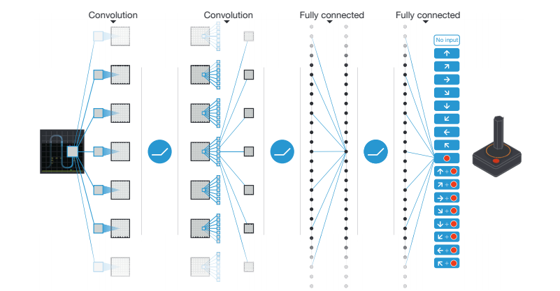
Below is a visualization of the convolutional neural network architecture from the paper, from which we can see it have:
- 3 convolutional layers (only 2 shown, 3 stated in the text)
- 2 linear layers
- ReLu activations between the first 3 layers
- The last layer is unactivated
The paper then discusses what to expect from the deep Q-learning algorithm when playing Atari games:
...our DQN agent performed at a level that was comparable to that of a professional human games tester across the set of 49 games, achieving more than 75% of the human score on more than half of the games
An important point is that this performance is without any input about the environment, meaning it is a completely model-free algorithm.
The exact architecture of the DQN agent is as follows:
- Input to the network is 84 x 84 x 4 image produced from preprocessing followed by a rectifier
- The second hidden layer convolves 64 filters of 4 3 4 with stride 2 followed by a rectifier
- The third convolutional layer convolves 64 filters of 3 x 3 x 3with stride 1 followed by a rectifier
- The final hidden layer is fully-connected and consists of 5 12 rectifier units
- The output layer is a fully-connected linear layer with a single output for each valid action (between 4 and 18 in the Atari games)
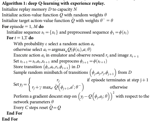
Below we can see the deep Q-learning algorithm that we're going to implement with PyTorch:
Now let's move on to preprocessing the images from OpenAI Gym Atari emulator.
Data Preprocessing
Preprocessing and stacking the frames from the OpenAI Atari environments is a critical to the success of the deep Q-learning agent.
The problems that we need to solve include:
- The images have 3 channels but our agent only needs 1 so we need to convert grayscale
- The images are quite large so we need to downscale them to 84 x 84 pixels
- The paper describes "flickering" of some objects in some environments - we solve this by keep track of the 2 previous frames and taking the max of the 2
- We repeat each action for 4 steps
- PyTorch expects images to have channels first, OpenAI returns channels last so we need to flip the axis of the Numpy arrays
- We need to stack the 4 most recent frames
- We need to scale the outputs by dividing the images by 255
In this step we really just need to keep in mind what data structures we need and what algorithms we want to implement.
We will start with the problem of taking the 2 previous frames and returning the max and then repeating each action for 4 steps.
We won't cover the preprocessing code in this article, but you can find useful pseudocode for preprocessing and the implementation on GitHub by Phil Tabor here.
Creating the Deep Q-Learning Agent's Memory
In this section we will create a mechanism for the agent to keep track of states, actions, rewards, new states, and the final state.
All of these factors will be used in the calculation of the Target for the loss function of the DQN.
For maximum flexibility of the agent the memory should accomodate states with an arbitrary shape.
We should also sample from the memory uniformly, meaning each memory will have an equal probability of being sampled, and we should not repeat memories.
In order to implement this in Python we can use either deques - which has the feature of adding and removing elements from either end - or Numpy arrays. In this implementation we'll use Numpy arrays.
Again we won't go over the code in this article, but you can find Phil Tabor's implementation of the replay memory here on Github.
The great part about this replay memory is that it can be reused for any Atari environment.
Building the Deep Q Network
Let's now build the deep Q network class, which will include the following:
- 3 convolutional layers and 2 fully connected layers
- A function to find the input size for the fully connected layer
- An RMSProp optimizer and MSE loss function
- Model checkpointing after every 100 records
A PyTorch implementation of the deep Q network from the course can be found on Github here.
Building the Deep Q Agent
Now that we have the replay memory and deep Q network class we can build the agent.
As discussed, one of the main innovations of deep Q-learning is that it is an online network that's updated with gradient descent in addition to a target network that calculates the target values.
The target network is updated periodically with the weights of the online network.
We also use a replay memory to sample the agent's history and trains the network.
The agent also needs functions for the following:
- A constructor called
DQNAgent - An epsilon-greedy action selection called
choose_selection - A function to copy the weights of the online network to the target network called
replace_target_network - A function to decrease epsilon over time called
decrement_epsilon - A function to learn from experiences called
learn - A function to store memories called
save_models - A function to interface with the deep Q network to save the model called
load_models
The implementation of the deep Q-learning agent in PyTorch by Phil Tabor can be found on Github here.
Building the Main Loop & Analyzing Performance
Now that we have the deep Q-learning agent we need to write a main loop and analyze performance.
We start by making the environment, which in this case will be 'PongNoFrameskip-v4'.
Next we instantiate a best_score to save the model when it acheives a new high score.
We will play 500 games for training and then instantiate the DQNAgent().
Next we load the checkpoint if appropriate, and then we define a filename for saving our plot at the end of training.
The main_dqn.py file by Phil Tabor can be found on Github here.
After running the code we can see we got an average score of ~16 points after running ~1 million learning steps. From the plot we can also see the agent learns as epsilon decreases but the majority of learning happens in the greedy phase.
From this deep Q-learning implementation we can see we get quite significant results in a short period of time and a (somewhat) rudimentary approach to the problem.
2. Double Q-Learning
Now that we have an implementation of deep Q-learning, we can expand on this and look at other papers.
Since we have the replay memory and preprocessing functionality we can simply tweak the agent as needed.
The next paper we'll review is called Deep Reinforcement Learning with Double Q-learning from Google DeepMind.
Again, we'll look at what algorithm we need to implement, the data structures we need, and the model architecture suggested by the authors.
Analyzing the Paper
As highlighted in the abstract, Q-learning is known to overestimate action values under certain conditions.
The paper says that such overestimations are common, can harm performance, alt0ugh they can generally be prevented.
The Double Q-learning algorithm is an adaption of the DQN algorithm that reduces the observed overestimation, and also leads to much better performance on several Atari games.
The reason the Q-learning can sometimes learn unrealistically high actions values is as follows:
...it includes a maximization step over estimated action values, which tends to prefer overestimated to underestimated values.
The issue that the authors highlight is that if this overestimation is not uniform and not concentrated on states that we want to learn more about (i.e. encouraging exploration), they might negatively affect the quality of the resulting policy.
The theory behind Double Q-learning is similar to deep Q-learning, although one of the main differences is that we can decouple the action selection from the evaluation.
In other words, as the authors state:
The idea of Double Q-learning is to reduce overestimations by decomposing the max operation in the target into action selection and action evaluation.
As described in the paper, in the original Double Q-learning algorithm:
...two value functions are learned by assigning each experience randomly to update one of the two value functions, such that there are two sets of weights, $\theta$ and $\theta^t$. For each update, one set of weights is used to determine the greedy policy and the other to determine its value.
In simple terms, as the name suggests instead of having a single Q-function we have two.
In order to implement this, all we need to change from our DQN algorithm is to modify the calculation of our target. The learning function, action function, etc. are all otherwise the same.
The Double DQN algorithm also uses the same network architecture as the original DQN.
Implementing Double Q-Learning with PyTorch
As mentioned, we can reuse much of the deep Q-learning code including the following functions:
- Networks
- Memory
- Action selection
- Network replacement
- Epsilon decrement
- Model saving
The difference with Double Q-learning is in the calculation of the target values.
The update equation for Double Q-learning from the paper is shown below:

The Double Q-learning implementation in PyTorch by Phil Tabor can be found on Github here.
3. Dueling Deep Q-Learning
Let's now look at one more deep reinforcement learning algorithm called Duelling Deep Q-learning.
Analyzing the Paper
The paper that we will look at is called Dueling Network Architectures for Deep Reinforcement Learning.
In the abstract of the paper the authors discuss how many deep reinforcement learning algorithms use conventional architectures such as convolutional networks, LSTMs, or autoencoders.
The architecture that they present is for model-free reinforcement learning. The dueling network has two separate estimators:
- One for the state value function
- And one for the state-dependent action advantage function
The authors describe the benefit of this architecture as follows:
The main benefit of this factoring is to generalize learning across actions without imposing any change to the underlying reinforcement learning algorithm.
The authors also highlight that this dueling architecture enables the RL agent to outperform the state-of-the-art on the Atari 2600 domain.
In the introduction the authors highlight that their approach can easily be combined with existing and future RL algorithms, so we won't have to make too many modifications to the code.
The authors specify the proposed network architecture as follows:
The dueling architecture consists of two streams that represent the value and advantage functions, while sharing a common convolutional feature learning module.
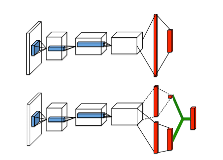
From the image above we see the popular Q-network on top and and the dueling Q-network on the bottom.
The authors go on to clarify how the architecture can be understood:
This dueling network should be understood as a single Q network with two streams that replaces the popular single-stream Q network in existing algorithms such as Deep Q-Networks
What this means is that the dueling architecture can learn the values of each state, without having to learn the effect of each action for each state.
Implementing Dueling Deep Q-Learning
In order to implement the dueling deep Q-learning algorithm we need to complete the following for the network:
- The convolutional layers are the same
- We need to split the linear layers into two steams: value & advantage stream
- We need to modify the feed forward function
We then need to complete the following for the agent class:
- Memory, target network updates, model saving, and epsilon decrementing are all the same
- Our action selection function needs an advantage stream
- We need to combine the value & advantage streams for the learn function
The dueling deep Q-learning network implemented in PyTorch by Phil Tabor can be found on GitHub here and the agent can be found here.
Summary: Deep Reinforcement Learning with PyTorch
As we've seen, we can use deep reinforcement learning techniques can be extremely useful in systems that have a huge number of states.
In these systems, the tabular method of Q-learning simply will not work and instead we rely on a deep neural network to approximate the Q-function.
We first looked at the naive deep Q-learning approach, and then reviewed several papers that solve the issue of correlations ruining the learning process, as well as the issue of using a single Q-function to both pick actions and update the weights of the network.
In particular, double Q-learning and dueling deep Q-learning are two interesting algorithms that solve these challenges.

