Introduction to the Capital Asset Pricing Model (CAPM) with Python

The Capital Asset Pricing Model (CAPM) is one of the most widely used formula in finance.

In this article, we'll first look at the theory and intuition behind CAPM and then we'll review how to calculate it with Python, both for an individual stock and a portfolio of stocks.

This article is based on notes from this course on Python & Machine Learning for Financial Analysis and is organized as follows:

• What is the Capital Asset Pricing Model (CAPM)?
• Capital Asset Pricing Model with Python
• Normalize & Visualize Data
• Calculate Daily Returns
• Calculate Beta for a Single Stock
• Calculate CAPM for a Single Stock
• Calculate Beta for a Portfolio of Stocks
• Calculate CAPM for a Portfolio of Stocks

What is the Capital Asset Pricing Model (CAPM)?

The Capital Asset Pricing Model (CAPM) describes the relationship between the expected return of assets and the systematic risk of the market.

CAPM indicates that the expected return of an asset is equal to the risk-free return plus a risk premium.  The assumption of CAPM is that investors are rational and want to maximize return and reduce risk as much as possible. The goal of CAPM is thus to calculate what return an investor can expect to make for a given risk premium over the risk-free rate.

Before we get to the CAPM formula, we first need to define a few variables.

Risk-Free Rate

CAPM also assumes there exists a risk-free asset $r_f$ with zero standard deviation. An example of a risk-free asset include Treasury Bills as they're backed by the U.S. government.

Market Return

The market return is denoted as $r_m$ and includes all securities in the market. A good representation of the U.S. market portfolio is the S&P 500, which is a market capitalization-weighted index of the 500 largest U.S. publicly traded companies.

Beta

Beta is a measure of a stock's volatility in relation to the overall market, for example the S&P 500. In other words, Beta represents the slope of the regression line, which is the market return vs. the individual stocks return.

Beta is used in the CAPM to describe the relationship between systematic risk, or market risk, and the expected return of an asset. By definition, we say that the overall market has a beta of 1.0 and individual stocks are ranked by how volatile they are relative to the market.

• If the Beta of an individual stock = 1.0, this means its price is perfectly correlated with the market
• If Beta < 1.0, which is referred to as 'defensive', this indicates the security is theoretically less volatile than the market
• If Beta > 1.0, or 'aggressive', this indicates the assets price is more volatile than the market

CAPM Formula

Mathematically, we can define CAPM formula as follows:

$$r_i = r_f + \beta_i(r_m - r_f)$$

where:

• $r_i$ is the expected return of a security
• $r_f$ is the risk free rate
• $\beta_i$ is the beta of the security relative to the market
• $r_m - r_f$ is the risk premium

Example of CAPM

Below is an example of the CAPM formula for Apple stock, where we'll make the following (made up) assumptions:

• The risk-free rate $r_1$ is 0%
• The market portfolio return $r_m$ is 12.4%
• The beta of Apple $\beta_i$ is 1.11

With these assumptions, we can calculate the CAPM of Apple as:

Expected return = 0% + 1.11(12.4% - 0%) = 13.7%

This formula suggests that an investor should expect a return of 13.7% in order to compensate for the additional risk they're taking.

Capital Asset Pricing Model with Python

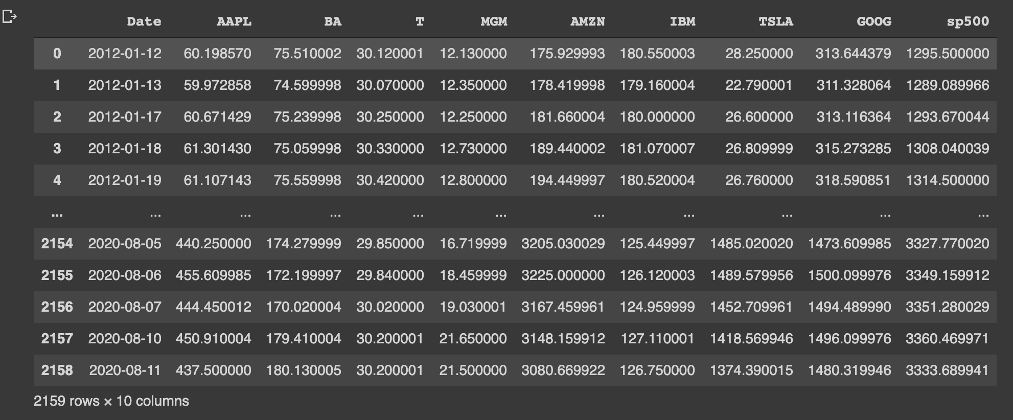
For this project we'll be using a CSV file of the following stocks prices from 2012 to 2020, sorted by date:

Normalize & Visualize Data

Next, we'll normalize our stock data with the following function, which loops through each column except the Date column and divides the price by the initial price:

# Normalize stock data based on initial price
def normalize(df):
  x = df.copy()
  for i in x.columns[1:]:
    x[i] = x[i]/x[i][0]
  return x

Next, we can plot the normalized prices using our normalize function with Plotly:

# Function to plot interactive plot
def interactive_plot(df, title):
  fig = px.line(title = title)
  for i in df.columns[1:]:
    fig.add_scatter(x = df['Date'], y = df[i], name = i)
  fig.show()

interactive_plot(normalize(stocks_df), 'Normalized Prices')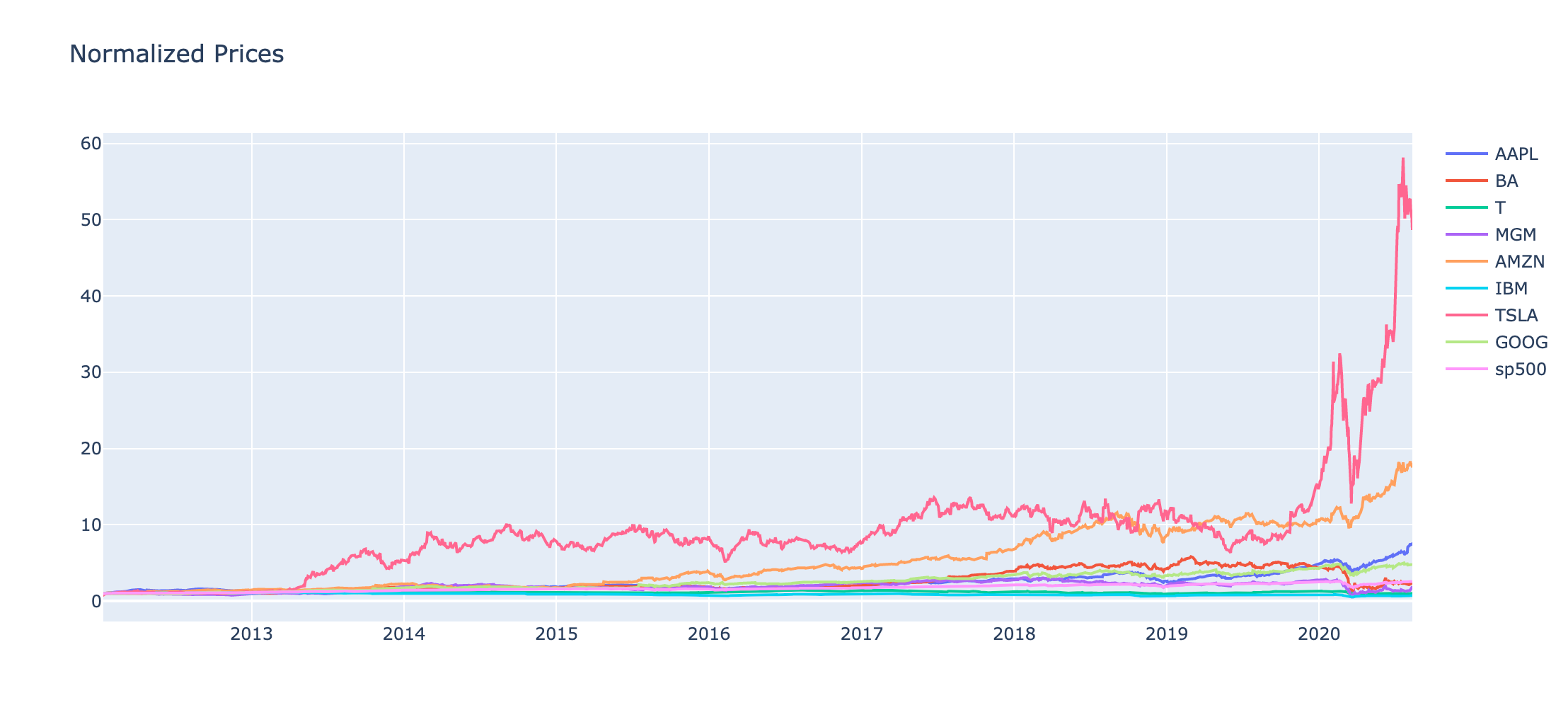

Calculate Daily Returns

Next we need to calculate the daily return of each stock with the daily_return function, which works as follows:

• Loops through each stock
• Loops through each row belonging to the stock
• Calculates the percentage of change from the previous day
• Sets the value of first row to zero, since there is no previous value

def daily_return(df):
  df_daily_return = df.copy()
    for i in df.columns[1:]:
        for j in range(1, len(df)):
            df_daily_return[i][j] = ((df[i][j]- df[i][j-1])/df[i][j-1]) * 100
        df_daily_return[i][0] = 0
  return df_daily_return

We then call the daily_return function on our stock dataset:

stocks_daily_return = daily_return(stocks_df)
stocks_daily_return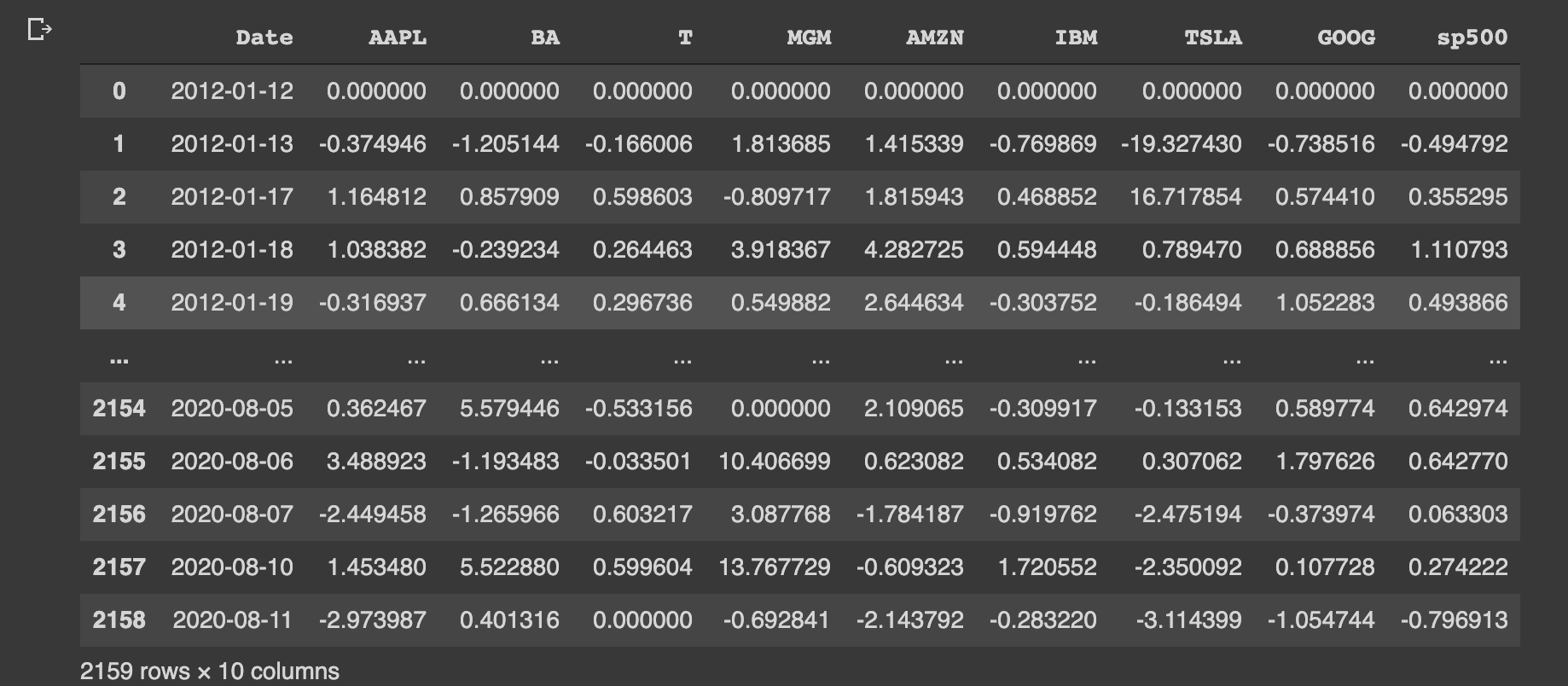

Calculate Beta for a Single Stock

Next we will calculate the beta and alpha of an individual stock relative to the S&P 500. To recap, beta is the slope of the line regression line, or the market return vs. stock return, which we can calculate with np.polyfit:

beta, alpha = np.polyfit(stocks_daily_return['sp500'], stocks_daily_return['AAPL'], 1)

Calculate CAPM for a Single Stock

Now that we have the daily returns and beta of a single stock, we can calculate the capital asset pricing model. First, we can calculate the average daily return of the market as follows:

stocks_daily_return['sp500'].mean()

We can then annualize this return by multiplying it by the number of trading days in a year:

rm = stocks_daily_return['sp500'].mean() * 252

Assuming a risk-free rate of 0, we can then calculate CAPM for AAPL using the formula discussed above:

rf = 0 
ER_AAPL = rf + (beta * (rm-rf)) 

Calculate Beta for a Portfolio of Stocks

Let's now look at calculating CAPM for the entire portfolio of stocks in this dataset.

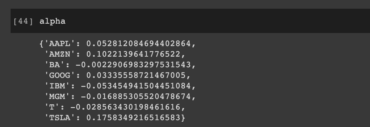
The first step is to create two empty dictionaries that will hold the beta and alpha of each stock. Alpha describes the strategy's ability to beat the market (S&P500):

beta = {}
alpha = {}

Next, we will loop through the daily returns of each stock and perform the following steps:

• We need to ignore the Date and S&P 500 columns
• Plot a scatter plot of each daily stock return and the daily market return
• Fit a polynomial line between each individual stock and the market and plot the best fit line
• Update the beta and alpha dictionaries

for i in stocks_daily_return.columns:
  if i != 'Date' and i != 'sp500':
    stocks_daily_return.plot(kind = 'scatter', x = 'sp500', y = i)
        b, a = np.polyfit(stocks_daily_return['sp500'], stocks_daily_return[i], 1)
        plt.plot(stocks_daily_return['sp500'], b * stocks_daily_return['sp500'] + a, '-', color = 'r')  
    beta[i] = b    
    alpha[i] = a  
    plt.show()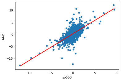

Below we can see the beta and alpha of each stock in the dataset:

Calculate CAPM for a Portfolio of Stocks

Now that we have the beta of each individual stock we can calculate the CAPM.

First, we will obtain a list with all the stock names called keys:

keys = list(beta.keys())

Next, we will define an empty dictionary for the expected returns of each individual stock. We'll also set the risk-free rate to 0 and get the annual return of the market:

ER = {}

rf = 0 
rm = stocks_daily_return['sp500'].mean() * 252 

Next we will create a for loop and apply the CAPM formula to each individual stock as follows:

for i in keys:
  ER[i] = rf + (beta[i] * (rm-rf)) 

Finally, we can print out the expected return based on CAPM of each stock:

Next, we will assign an equal weight to each stock in the portfolio. We can then calculate the expected portfolio return by multiplying the portfolio_weights  by the sum of expected returns for the individual stocks:

portfolio_weights = 1/8 * np.ones(8) 
ER_portfolio = sum(list(ER.values()) * portfolio_weights)

The expected return based on CAPM for the portfolio is roughly 13%:

Summary: Capital Asset Pricing Model with Python

In this article we reviewed how to calculate the Capital Asset Pricing Model (CAPM) with Python. We first defined several key variables that we need for the CAPM formula including the risk-free rate of return, the market return, and beta.

We then looked at how to calculate the daily returns for each stock, calculate the beta of an individual stock, and apply the CAPM formula. Finally, we looked at how to use the CAPM formula for an entire portfolio of stocks.

Resources

• Python & Machine Learning for Financial Analysis