AI for Ecommerce: Optimizing Business Processes with Reinforcement Learning

Regardless of the type of business you're in, the three main practical applications of AI are:

• Optimizing business processes
• Minimizing costs
• Maximizing revenue

In this article we're going to look at an example of optimizing business processes for an eCommerce warehouse. We're going to do this by creating an autonomous robot that can navigate the warehouse and pick up products in the most efficient way possible.

To do this we're going to make use of reinforcement learning, specifically Q-learning.

We won't cover the theory and intuition of Q-learning and reinforcement learning in this article as we've covered it extensively, but if you need a refresher before continuing check out the articles below:

• What is Reinforcement Learning? A Complete Guide for Beginners
• Deep Reinforcement Learning: Guide to Deep Q-Learning

This article is based on notes from this course on Artificial Intelligence for Business and is organized as follows:

1. Project Overview
2. Defining the Environment
3. Python Implementation of Q-Learning for Optimization

1. Project Overview

As mentioned, for this project we're going to optimize the flows of a warehouse for an eCommerce company.

We can think of the warehouse like a maze, and for this example we're going to say that there are 12 product categories stored in 12 unique locations.

As orders are placed online, we want our autonomous robot to find and retrieve the product from one of the 12 locations.

To do this, the robot will make use of two systems:

• The first is not AI, but will rank in real-time the priority of each product to be collected and the corresponding location
• The second is our Q-learning agent, which will compute the shortest distance from its current location to the top priority location

In order to solve this problem, we first need to define the environment, which involves defining the states, actions, and rewards for our agent.

We will then work through the implementation of our reinforcement learning agent in Python.

2. Defining the Environment

For any reinforcement learning problem we're working on, we first need to define the states, actions, and rewards of environment.

First let's briefly review these terms:

• A state is the input for our model
• The model then takes the state as input and returns an output, which is our action
• The model then takes the state and action as input and returns the reward as output

State

In our case, the state is going to be the location of the robot at a given time $t$. Since we have 12 locations, we will have 12 input states from 0 - 11.

Action

The action is the next possible location that the agent can go, so again the actions will be from 0 - 11.

Since there are walls in the warehouse not every location can be the next possible action, so we'll need to create a function to return the possible actions given the layout of the warehouse.

Reward

Since we have a finite number of states and a finite number of actions, we will define our reward as a matrix where the rows correspond to the states and the columns correspond to the action.

The reward will either be a 1 if in the given state we can take an action that get's us to our final location, or 0 if we need to go through another location first to get to our destination.

We'll then set a large reward for our final destination, so that the agent learns to go to that one.

3. Python Implementation of Q-Learning for Optimization

Let's now look at how we can implement Q-learning in Python to optimize the eCommerce warehouse flows.

To recap, we want to build a model that takes in the robots current location at time $t$ and returns the optimal route to retrieve the top priority product.

We're first going to look at one top priority at a time, and then we'll add the option to use intermediary steps to pick up other high priority products along the way.

We're going to make use of Google Colab for this project, and as usual the first step is to import our libraries. In this case, we only need Numpy:

import numpy as np

Next we need to set the parameters for our implementation, and since we're dealing with Q-learning we have two important parameters:

• $\gamma$ - gamma is the discount factor in the Temporal Difference
• $\alpha$ - alpha is the learning rate for the Bellman equation

# Set the parameters gamma & alpha for Q-learning
gamma = 0.75
alpha = 0.9

We're now ready to:

• Define the environment
• Build and train the model with Q-learning
• Go into production with our model

Step 1: Defining the Environment

As discussed, to define the environment we need to define the states, actions, and rewards.

To define the states we're going to create a dictionary that maps the letters associated with each of the 12 locations to the states and indexes:

# Define the states
location_to_state = {'A': 0,
                    'B': 1,
                    'C': 2,
                    'D': 3,
                    'E': 4,
                    'F': 5,
                    'G': 6,
                    'H': 7,
                    'I': 8,
                    'J': 9,
                    'K': 10,
                    'L': 11,}

Recall that we specify the actions that can't be taken with a 0 in our reward matrix and 1 for an action that can be taken.

So the actions are the indexes of the 12 locations:

# Define the actions:
actions = [0,1,2,3,4,5,6,7,8,9,10,11]

To define the rewards we need to define a reward function that takes as input the the state-action pair at a given time $t$ and return the reward we get by playing that action in the state:

\[R: (s_t \ \epsilon \ S, a_t \ \epsilon \ A) \mapsto r_t \ \epsilon \ R\]

As mentioned, with a finite number of states and actions the best way to define the reward function is to create a matrix with the states as rows and actions as columns.

If you want to see the layout for this specific warehouse you can find it in the AI for Business course, but for now here is the 2D Numpy array we will use:

# Define the rewards
R = np.array([[0,1,0,0,0,0,0,0,0,0,0,0],
              [1,0,1,0,0,1,0,0,0,0,0,0],
              [0,1,0,0,0,0,1,0,0,0,0,0],
              [0,0,0,0,0,0,0,1,0,0,0,0],
              [0,0,0,0,0,0,0,0,1,0,0,0], 
              [0,1,0,0,0,0,0,0,0,1,0,0], 
              [0,0,1,0,0,0,1,1,0,0,0,0],
              [0,0,0,1,0,0,1,0,0,0,0,1],
              [0,0,0,0,1,0,0,0,0,1,0,0],
              [0,0,0,0,0,1,0,0,1,0,1,0],
              [0,0,0,0,0,0,0,0,0,1,0,1],
              [0,0,0,0,0,0,0,1,0,0,1,0]])

We're now ready to start building and training the AI model with Q-learning.

Step 2: Building & Training the Model with Q-Learning

It's now time to implement each step of the Q-learning algorithm.

The steps we need to implement include:

• Initializing the Q-values
• Write a for loop for our Q-learning process over 1000 iterations

We first need to initialize all the different states-action pairs to 0. To do this we create a Q-function that takes as input the state-action pair and returns the Q-value.

Again, since we have a finite number of states and actions the best way to do this is to create a matrix of Q-values initialized with 0's.

Instead of typing out all the 0's we can make use of Numpy's built-in np.zeros function:

# Initializing the Q-Values
Q = np.array(np.zeros([12,12]))

Now we need to write a for loop with 1000 iterations for the Q-learning algorithm.

To implement the Q-learning process we need to:

1. Select a random state $s_t$ from our 12 possible states

2. Play a random action $a_t$ that will lead to the next state, such that $R(s_t, a_t) > 0$. Recall that we need to only play certain actions in our current state, so we need to write a function for that. To do this create an empty list called playable_actions and write another for loop to loop through our matrix and find the 1's

3. When we reach the next step we get a reward $R(s_t, a_t)$. We do this by just setting a variable next_state equal to our action.

4. We compute the Temporal Difference $TD(s_t, a_t)$. The Temporal difference is the difference between the reward we get by playing action $a_t$ in state $s_t$ plus the highest Q-value of the next state minus the Q-value of the action played in the current state. Temporal difference is given by this formula:

\[TD_t(s_t, a_t) = R(s_t, a_t) + \gamma \ max_a(Q(s_{t+1}, a)) - Q(s_t, a_t)\]

5. We update the Q-value by applying the Bellman equation, which is given by the following formula:

\[Q_t(s_t, a_t) = Q_{t-1}(s_t, a_t) + \alpha TD_t(s_t, a_t)\]

# Implement the Q-learing Process over 1000 iterations
for i in range(1000):
  
  # Select a random state
  current_state = np.random.randint(0, 12)
  
  # Find a list of playable actions
  playable_actions = []
  for j in range(12):
    if R[current_state, j] > 0:
      playable_actions.append(j)
  
  # Play a random action and go to the next state
  next_state = np.random.choice(playable_actions)
  
  # Compute the Temporal Difference
  TD = R[current_state, next_state] + gamma * Q[next_state, np.argmax(Q[next_state,])] - Q[current_state, next_state]
  
  # Update the Q-value by applying the Bellman equation
  Q[current_state, next_state] += alpha * TD 

Now that we have our Q-learning implementation let's go into production with the model.

Step 3: Going into Production

To go into production we're going write a function that takes as input the starting location of the robot and the final location, which is the top priority location.

This function will return the most efficient path for the robot to take, and this will be learned through the Q-values computed from our model.

The route will be returned in the form of a list of successive locations that we need to go through from start to finish.

Both the inputs and outputs of the function will be in letters for our 12 locations from A to L.

To start we're going to assume we're already at location E and we want to go to location G.

We can first manually specify that we want to go to location G by setting a high reward at that location.

On our reward matrix that corresponds to the 7th row and 7th column, so we'll set that reward to 1000 as shown below:

# Define the rewards
R = np.array([[0,1,0,0,0,0,0,0,0,0,0,0],
              [1,0,1,0,0,1,0,0,0,0,0,0],
              [0,1,0,0,0,0,1,0,0,0,0,0],
              [0,0,0,0,0,0,0,1,0,0,0,0],
              [0,0,0,0,0,0,0,0,1,0,0,0], 
              [0,1,0,0,0,0,0,0,0,1,0,0], 
              [0,0,1,0,0,0,1000,1,0,0,0,0],
              [0,0,0,1,0,0,1,0,0,0,0,1],
              [0,0,0,0,1,0,0,0,0,1,0,0],
              [0,0,0,0,0,1,0,0,1,0,1,0],
              [0,0,0,0,0,0,0,0,0,1,0,1],
              [0,0,0,0,0,0,0,1,0,0,1,0]])

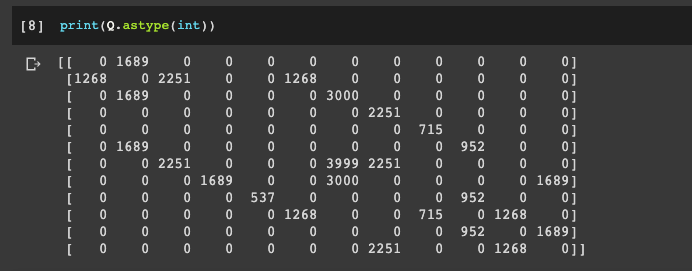
Here's what we get when we print our Q-values with print(Q.astype(int)):

From this matrix that row G and column G has the highest value, and the other high Q-values are locations that get you closer to G.

Now you can see to take this into production we are going to write a function that takes in the initial location, then checks the highest Q-value in the row and plays that action.

The action leads us to the next state where we repeat the process until we get closer and closer to the highest value location.

We're now ready to write the function called route that will take in the starting and ending location and return the optimal route.

As mentioned, this function will return a list of successive locations that the robot needs to go through to reach the final location.

Here are the steps we need to take to create this function:

• We're going to create a variable called route that we will initialize with a list with one element: the starting location.
• To find the next location we're going to write a while loop - we use this instead of a for loop since we don't know how many iterations it will take to get to the final location
• Before writing our while loop we need to introduce a variable for the next_location - at first we don't know what this is so we set it to starting_location and then we'll compute it with the matrix of Q-values
• The first thing we need in our while loop is to convert the letter from our starting location into the index of the row. We call this variable starting_state and we're going to use our location_to_state dictionary from earlier.
• Now that we have the row the next step is to figure out the maximum Q-value of that row with the np.argmax function
• Since we want to return our route as successive letters instead of indexes we need to do an inverse mapping from numbers to letters. Instead of putting this mapping in the function we will add it before the function, and we can do this with a for loop inside of the dictionary to inverse our earlier dictionary.
• Next we update our next_location variable using our state_to_location dictionary and passing in our next_state
• Finally we need to append our route with the next_location and then we need to end the while loop by updating our starting_location with the next_location.

# Mapping from states to location
state_to_location = {state: location for location, state in location_to_state.items()}

# Function that returns the optimal route
def route(starting_location, ending_location):
  route = [starting_location]
  next_location = starting_location
  while (next_location != end):
    starting_state = location_to_state[starting_location]
    next_state = np.argmax(Q[starting_state,])
    next_location = state_to_location[next_state]
    route.append(next_location)
    starting_location = next_location
  return route

To check the function let's print the final route from location E to G:

Before we finish, it would be better if we can update our route function to automatically change the rewards of our final locations, instead of manually updating it.

To do this we're going to create a copy of our matrix of rewards since we always want to leave our initial reward matrix the same. We can use Numpy for this with R_new = np.copy(R).

Now we take this copy and map the ending_location to the ending_state with our location_to_state dictionary. We then update the reward of the desired cell by setting this row and column to 1000:

# Make a function that returns the optimal route
def route(starting_location, ending_location):
  R_new = np.copy(R)
  ending_state = location_to_state[ending_location]
  R_new[ending_state, ending_state] = 1000
  route = [starting_location]
  next_location = starting_location
  while (next_location != ending_location):
    starting_state = location_to_state[starting_location]
    next_state = np.argmax(Q[starting_state,])
    next_location = state_to_location[next_state]
    route.append(next_location)
    starting_location = next_location
  return route

There is one more important step to take - since the Q-learning happens on R before we make the R_new updated copy, so we need to integrate the Q-learning process into the route function:

# Mapping from states to location
state_to_location = {state: location for location, state in location_to_state.items()}

# Make a function that returns the optimal route
def route(starting_location, ending_location):
  R_new = np.copy(R)
  ending_state = location_to_state[ending_location]
  R_new[ending_state, ending_state] = 1000
  Q = np.array(np.zeros([12,12]))
  
# Implement the Q-learing Process over 1000 iterations
  for i in range(1000):  
  # Select a random state
    current_state = np.random.randint(0, 12) 
  # Find a list of playable actions
    playable_actions = []
    for j in range(12):
      if R_new[current_state, j] > 0:
        playable_actions.append(j)
    # Play a random action and go to the next state
    next_state = np.random.choice(playable_actions) 
    # Compute the Temporal Difference
    TD = R_new[current_state, next_state] + gamma * Q[next_state, np.argmax(Q[next_state,])] - Q[current_state, next_state]
    # Update the Q-value by applying the Bellman equation
    Q[current_state, next_state] += alpha * TD 
  
  route = [starting_location]
  next_location = starting_location
  while (next_location != ending_location):
    starting_state = location_to_state[starting_location]
    next_state = np.argmax(Q[starting_state,])
    next_location = state_to_location[next_state]
    route.append(next_location)
    starting_location = next_location
  return route

After printing out the optimal route we can see we get the same path as earlier.

Summary: Optimizing Business Processes with Reinforcement Learning

In this article we looked at a practical example of how reinforcement learning can be used to optimize business processes.

Specifically, we used Q-learning to train an autonomous robot how to choose the most efficient route to pick up products.

To solve this problem with first defined the environment, including the states, actions, and rewards for our agent.

We then implemented this in Python and built a model that takes in the robots current location at time $t$ and returned the optimal route to retrieve the top priority product.

In the next article on AI for Ecommerce we're going to look look at an example of maximizing revenue with another reinforcement learning algorithm called Thompson Sampling.

Stay tuned.

Resources

• Artificial Intelligence for Business